Assignment 4 Solutions: Predicates and Measures

1. Load the cejst_nw.shp use the correct predicates to determine whether the geometries are valid and to check for empty geometries. If there are empty geometries, determine which rows have empty geometries (show your code).

Remember that predicates return logical (i.e. TRUE or FALSE) answers so we are looking for functions with st_is_* to look for valid or empty geometries. We wrap those in the all() or any() function calls so that we get a single TRUE or FALSE for the entire geometry collection rather than returning the value for each individual observation. While those can be useful for figuring out if the entire dataset meets our criteria (i.e., all are valid or any have empty geometries), identifying which records have empty geometries takes an additional step. We use which() to return the row index of each record that returns a TRUE for st_is_empty() and then subset the original data using the [] notation keeping only the rows with empty geometries and all other columns.

library(sf)
library(tidyverse)
library(terra)

cejst.nw <- read_sf("opt/data/data/assignment04/cejst_nw.shp")
all(st_is_valid(cejst.nw))
any(st_is_empty(cejst.nw))
which(st_is_empty(cejst.nw))

cejst.nw[which(st_is_empty(cejst.nw)),]

2. Load the landmarks_ID.csv table and convert it to an sf object. Now filter to just the hospital records (MTFCC == "K1231") and calculate the distance between all of the hospitals in Idaho. Note that you’ll have to figure out the CRS for the landmarks dataset…

Here we are interested in distance which is a measure (not a predicate or transformer), but to get there we need to take a few extra steps. First, we read in the csv file and convert it to coordinates (using st_as_sf, a transformer). Then we use dplyr::filter to retain only the hospitals in the dataset. Finally, because this is a lat/long dataset, we assume a geodetic projection of WGS84 and assign it to the filtered object. Once we’ve gotten all that squared away, it’s just a matter of using the st_distance function to return the distance matrix for all objects in the dataset.

hospitals.id <- read_csv("opt/data/data/assignment04/landmarks_ID.csv") %>% 
  st_as_sf(., coords = c("longitude", "lattitude")) %>% 
  filter(., MTFCC == "K1231")
st_crs(hospitals.id) <- 4326

dist.hospital <- st_distance(hospitals.id)

dist.hospital[1:5, 1:5]

3. Filter the cejst_nw.shp to just those records from Ada County. Then filter again to return the row with the highest annual loss rate for agriculture (2 hints: you’ll need to look at the columns.csv file in the data folder to figure out which column is the expected agricultural loss rate and you’ll need to set na.rm=TRUEwhen looking for the maximum value). Calculate the area of the resulting polygon.

This one should be relatively straightforward. We start with another call to dplyr::filter to get down to just the tracts in Ada County (note the use of the & to combine two logical calls). Then we use a second filter to return the row with the max value for agricultural loss. Note that we have to use the na.rm=TRUE argument to avoid having the NA values force the function to return NA.

ada.cejst <- cejst.nw %>% 
  filter(., SF == "Idaho" & CF == "Ada County") 

ada.max.EALR <- ada.cejst %>%  
  filter(., EALR_PFS == max(EALR_PFS, na.rm = TRUE))
  
ada.max.EALR[, c("SF", "CF", "EALR_PFS")]

Simple feature collection with 1 feature and 3 fields
Geometry type: MULTIPOLYGON
Dimension:     XY
Bounding box:  xmin: -116.1998 ymin: 43.11297 xmax: -115.9742 ymax: 43.59134
Geodetic CRS:  WGS 84
# A tibble: 1 × 4
  SF    CF         EALR_PFS                                             geometry
  <chr> <chr>         <dbl>                                   <MULTIPOLYGON [°]>
1 Idaho Ada County      0.7 (((-116.1371 43.55217, -116.137 43.55222, -116.1369…

4. Finally, look at the helpfile for the terra::adjacent command. How do you specify which cells you’d like to get the adjacency matrix for? How do you return only the cells touching your cells of interest? Use the example in the helpfile to illustrate how you’d do this on a toy dataset - this will help you learn to ask minimally reproducible examples.

We can access the helpfile for adjacent by using ?terra::adjacent (I won’t do that here because I don’t want to print the entire helpfile). From that we can see that the cells argument is the place to specify which cells we are interested in. also see that the directions argument allows us to specify whether we want “rook”, “bishop”, or “queen” neighbors. Finally, we see that if we want to exclude the focal cell itself, we have to set include to FALSE. By plotting the map with the cell numbers, we can see that cells 1 and 5 are on th top row of the raster and thus do not have any neighbors for for the upper 3 categories whereas cell 55 has all 8 neighbors. If you choose cells that are in the center of the raster, you get all neighbors

r <- rast(nrows=10, ncols=10)
cellnum <- cells(r)
r[] <- cellnum
plot(r)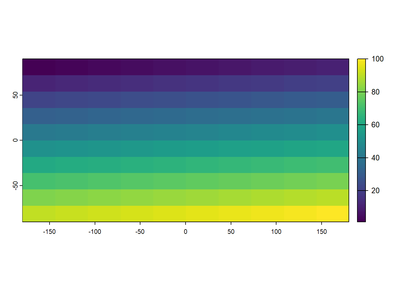

adjacent(r, cells=c(1, 5, 55), directions="queen", include=FALSE)

   [,1] [,2] [,3] [,4] [,5] [,6] [,7] [,8]
0   NaN  NaN  NaN   10    2   20   11   12
4   NaN  NaN  NaN    4    6   14   15   16
54   44   45   46   54   56   64   65   66

adjacent(r, cells=c(51, 52, 55), directions="queen", include=FALSE)

   [,1] [,2] [,3] [,4] [,5] [,6] [,7] [,8]
50   50   41   42   60   52   70   61   62
51   41   42   43   51   53   61   62   63
54   44   45   46   54   56   64   65   66