── Conflicts ────────────────────────────────────────── tidyverse_conflicts() ──
✖ tidyr::extract() masks terra::extract()
✖ dplyr::filter()  masks stats::filter()
✖ dplyr::lag()     masks stats::lag()
ℹ Use the conflicted package (<http://conflicted.r-lib.org/>) to force all conflicts to become errors
library(tidycensus)library(tmap)
Breaking News: tmap 3.x is retiring. Please test v4, e.g. with
remotes::install_github('r-tmap/tmap')
# load data# get a selection of 1000 Venus flytrap observations from rgbifvflytrap_us <-occ_search(scientificName ="Dionaea muscipula", country ="US",hasCoordinate =TRUE,limit=1000)# geodata rastersoils <- geodata::soil_world(var ="nitrogen", depth=5, path=tempfile())# boundariesstate_boundaries <- geodata::gadm(country ="USA", level=1, path=tempfile())
Write pseudocode for how you will prepare your data for visualization, then execute your plan. Some possible objectives might be cropping your data to an area of interest and transforming the data to tidy format.
There are a few necessary steps before I can plot. First, all vector data needs to be an sf object. rgbif returns a non-spatial dataframe, so I need to convert that to a spatial object. Next, I know Venus flytraps are endemic to just a few US states, so I will use spatial cropping tools to focus all my datasets to that area of interest. Finally, I convert my raster data to a dataframe. I always make this my last step before plotting, as I cannot perform any more spatial operations on the non-spatial dataframe.
1. Convert Venus flytrap data to spatial object2. Convert state boundaries from SpatVector to sf object3. Filter state boundaries to only include North and South Carolina4. Subset Venus flytrap data to those states5. Crop soils raster to those states6. Convert soils raster to data frame
# Convert Venus flytrap data to spatial objectvflytrap_us <- vflytrap_us$datavflytrap_dat_sf <- vflytrap_us %>%filter(!is.na(decimalLatitude) &!is.na(decimalLongitude)) %>%st_as_sf(coords =c("decimalLongitude", "decimalLatitude"), crs =4326)# Convert state boundaries from SpatVector to sf objectaoi <-st_as_sf(state_boundaries) %>%# Filter state boundaries to only include North and South Carolinafilter(NAME_1 %in%c("North Carolina", "South Carolina"))# Subset Venus flytrap data to those statesvflytrap_sub <-st_crop(vflytrap_dat_sf, aoi)
Warning: attribute variables are assumed to be spatially constant throughout
all geometries
# Crop soils raster to those statessoils_plot <-crop(soils, aoi, mask=TRUE) %>%# Convert soils raster to data frameas.data.frame(soils, xy=TRUE)
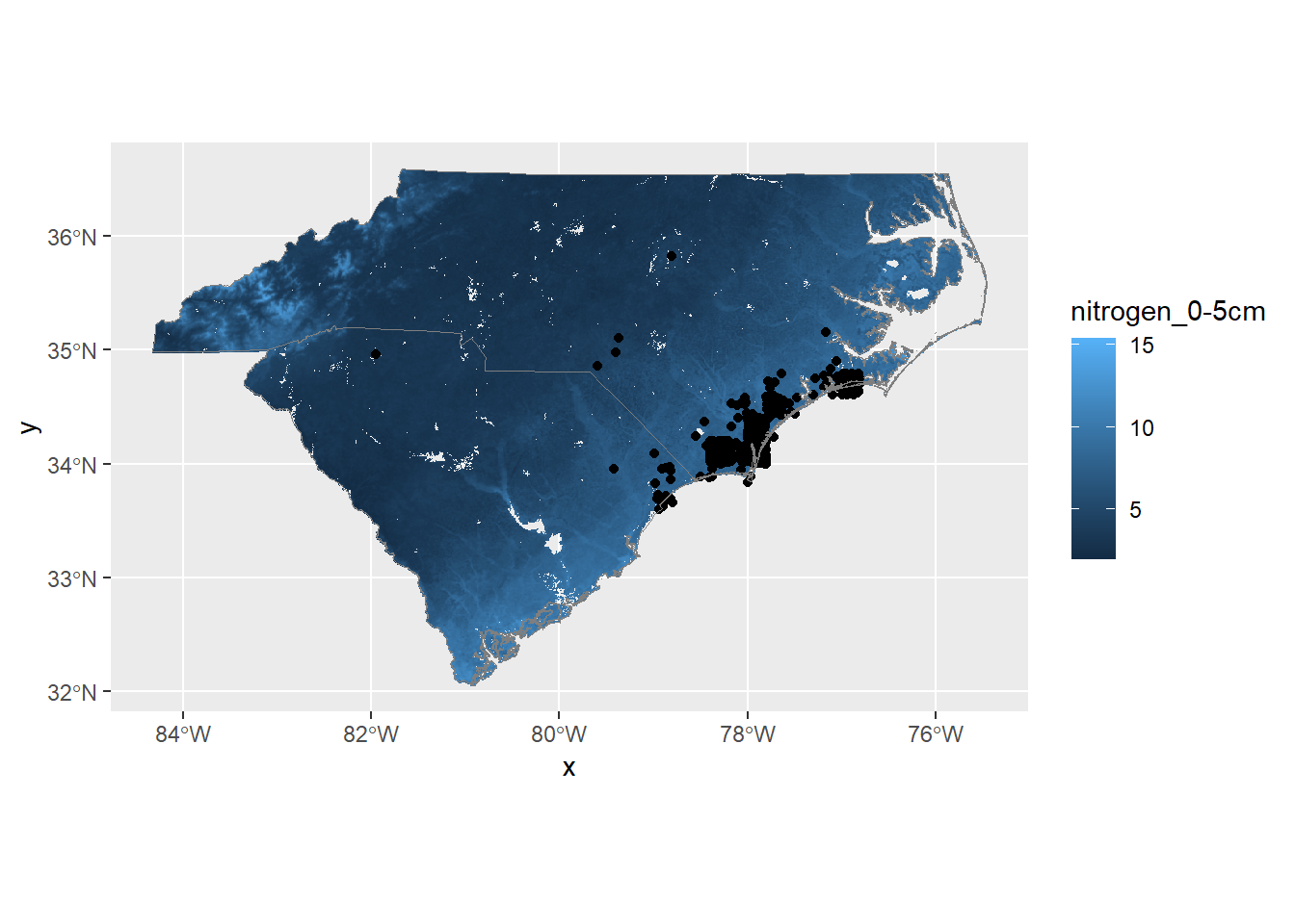
Use ggplot2 to create a map of the raster data with the species presence points overlayed on top. Add state/province/equivalent level boundaries.
First, I plot the raster. Then, I overlay the points and then the state polygons. coord_sf() is optional since ggplot2 can retrieve the correct coordinate system from the sf data.
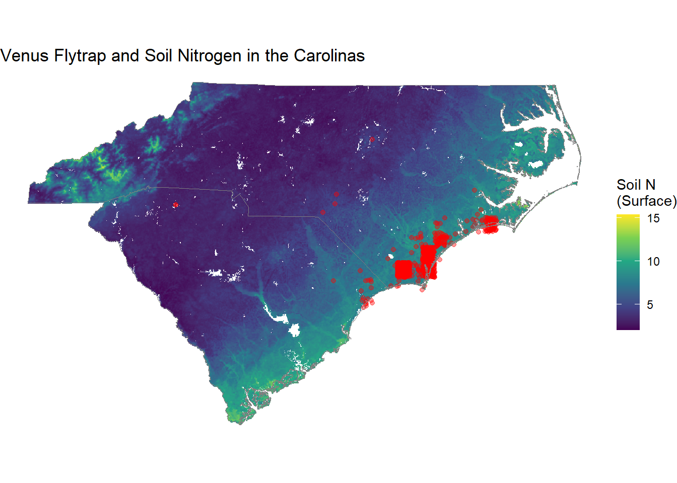
Change the raster color scale, legend name, title, and theme from ggplot2 defaults. You can try any other ggplot customization you’d like now as well.
The color scale and legend name can be changed in the scale_fill_* function. I like the viridis scale, so I’ll use that here. The plot title can be changed in labs. I’d like to get rid of the gray background and axes, so I’ll use theme_void. I’ll also make the points slightly transparent and bright red for better visualization.
ggplot() +geom_raster(data = soils_plot, aes(x=x, y=y, fill=`nitrogen_0-5cm`)) +geom_sf(data=vflytrap_sub, alpha =0.4, color="red") +geom_sf(data=aoi, color="gray50", fill=NA) +scale_fill_viridis_c(name ="Soil N\n(Surface)") +labs(title ="Venus Flytrap and Soil Nitrogen in the Carolinas") +theme_void()
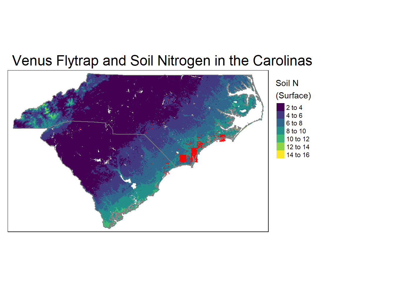
Use tmap to recreate this plot with zooming functionality and any other interactive elements you’d like to add. Optionally, you can substitute the raster for tidycensus or other polygon data at this stage.
First, I’ll use tmap to recreate the plot above.
tm_shape(crop(soils, aoi, mask=TRUE)) +tm_raster(n=8, palette = viridis::viridis(8),title ="Soil N\n(Surface)") +tm_legend(outside=TRUE) +tm_shape(vflytrap_sub) +tm_dots(alpha=0.4, col="red") +tm_shape(aoi) +tm_borders("gray50") +tm_layout(main.title="Venus Flytrap and Soil Nitrogen in the Carolinas")
Zoom capabilities are possible with tmap_mode. The default hover text is the first column in vflytrap_sub, which is the specimen key. This could be helpful, but I’m going to change it to the year of observation.
tmap_mode("view")tm_shape(crop(soils, aoi, mask=TRUE)) +tm_raster(n=8, palette = viridis::viridis(8),title ="Soil N\n(Surface)") +tm_legend(outside=TRUE) +tm_shape(vflytrap_sub) +tm_dots(alpha=0.4, id="year", col="red") +tm_shape(aoi) +tm_borders("gray50") +tm_layout(main.title="Venus Flytrap and Soil Nitrogen in the Carolinas")
For a tidycensus example, I’ll pull data on county level population to see if Vensus flytraps are in heavily populated areas.
block_pop <-get_acs(geography ="county",# most recent year availableyear =2022,variables ="B01001_001",state =c("NC", "SC"),geometry=TRUE)block_pop_proj <- block_pop %>%st_make_valid() %>%filter(!st_is_empty(.)) %>%st_transform(crs =st_crs(vflytrap_sub))tm_shape(block_pop_proj) +tm_polygons(col="estimate", border.alpha =0,n=8, palette = viridis::viridis(8),title ="Population", id="estimate") +tm_legend(outside=TRUE) +tm_shape(vflytrap_sub) +tm_dots(alpha=0.4, col="red", interactive=FALSE) +tm_shape(aoi) +tm_borders("gray50") +tm_layout(main.title="Venus Flytrap and Population in the Carolinas")