Session 14 code

Author

Carolyn Koehn

Libraries for today:

Code

library(tidyverse, quietly = TRUE)
library(spData)
library(sf)

Subsetting Data:

Code

colnames(world)

 [1] "iso_a2"    "name_long" "continent" "region_un" "subregion" "type"     
 [7] "area_km2"  "pop"       "lifeExp"   "gdpPercap" "geom"

Code

head(world)[,1:3] %>% 
  st_drop_geometry()

# A tibble: 6 × 3
  iso_a2 name_long      continent    
* <chr>  <chr>          <chr>        
1 FJ     Fiji           Oceania      
2 TZ     Tanzania       Africa       
3 EH     Western Sahara Africa       
4 CA     Canada         North America
5 US     United States  North America
6 KZ     Kazakhstan     Asia

Code

world %>%
  dplyr::select(name_long, continent) %>%
  st_drop_geometry() %>% 
  head(.)

# A tibble: 6 × 2
  name_long      continent    
  <chr>          <chr>        
1 Fiji           Oceania      
2 Tanzania       Africa       
3 Western Sahara Africa       
4 Canada         North America
5 United States  North America
6 Kazakhstan     Asia

Code

head(world)[1:3, 1:3] %>% 
  st_drop_geometry()

# A tibble: 3 × 3
  iso_a2 name_long      continent
* <chr>  <chr>          <chr>    
1 FJ     Fiji           Oceania  
2 TZ     Tanzania       Africa   
3 EH     Western Sahara Africa

Code

world %>%
  filter(continent == "Asia") %>% 
  select(name_long, continent) %>%
  st_drop_geometry() %>% 
  head(.)

# A tibble: 6 × 2
  name_long   continent
  <chr>       <chr>    
1 Kazakhstan  Asia     
2 Uzbekistan  Asia     
3 Indonesia   Asia     
4 Timor-Leste Asia     
5 Israel      Asia     
6 Lebanon     Asia

Create new columns

Code

world_dens <- world %>%
  filter(continent == "Asia") %>% 
  select(name_long, continent, pop, gdpPercap ,area_km2) %>%
  mutate(., dens = pop/area_km2,
         totGDP = gdpPercap * pop) %>%
  st_drop_geometry() %>% 
  head(.)

Aggregate / Summarise

Code

world %>%
  st_drop_geometry(.) %>% 
  group_by(continent) %>%
  summarize(pop = sum(pop, na.rm = TRUE))

# A tibble: 8 × 2
  continent                      pop
  <chr>                        <dbl>
1 Africa                  1154946633
2 Antarctica                       0
3 Asia                    4311408059
4 Europe                   669036256
5 North America            565028684
6 Oceania                   37757833
7 Seven seas (open ocean)          0
8 South America            412060811

Joins

Code

head(coffee_data)

# A tibble: 6 × 3
  name_long                coffee_production_2016 coffee_production_2017
  <chr>                                     <int>                  <int>
1 Angola                                       NA                     NA
2 Bolivia                                       3                      4
3 Brazil                                     3277                   2786
4 Burundi                                      37                     38
5 Cameroon                                      8                      6
6 Central African Republic                     NA                     NA

Code

world_coffee = left_join(world, coffee_data)

Joining with `by = join_by(name_long)`

Code

nrow(world_coffee)

[1] 177

Code

plot(world_coffee["coffee_production_2016"])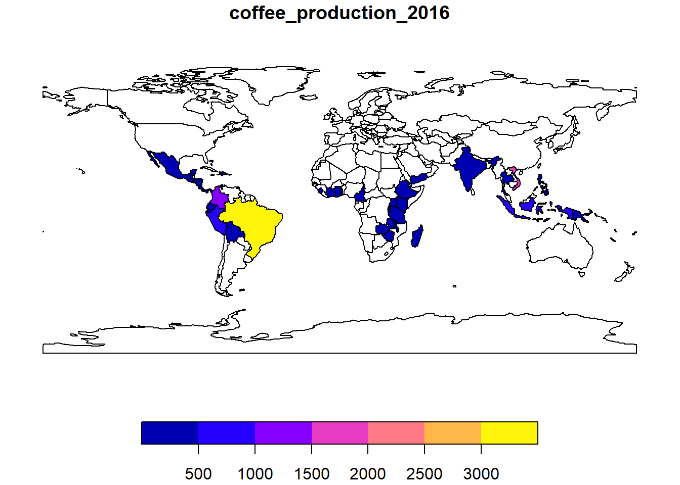

Code

world_coffee_inner = inner_join(world, coffee_data)

Joining with `by = join_by(name_long)`

Code

nrow(world_coffee_inner)

[1] 45

Practice:

What is the population density for the tracts in the cejst data? Our data sources are:

Total population in each tract (cejst$TPF)
Area in $m^2$ of each tract (tigris::tracts(), column ALAND)

Code

cejst <- st_read("/opt/data/data/assignment06/cejst_pnw.shp")

id_tracts <- tigris::tracts(state = "ID", year = 2015)

Code

cejst_id <- cejst %>%
  filter(SF == "Idaho")

Code

id_tracts <- id_tracts %>%
  mutate(ALAND_sqmi = ALAND/2589988.11)
head(id_tracts)

Simple feature collection with 6 features and 13 fields
Geometry type: POLYGON
Dimension:     XY
Bounding box:  xmin: -117.0628 ymin: 41.99601 xmax: -111.5077 ymax: 46.39597
Geodetic CRS:  NAD83
  STATEFP COUNTYFP TRACTCE       GEOID    NAME             NAMELSAD MTFCC
1      16      041  970200 16041970200    9702    Census Tract 9702 G5020
2      16      041  970100 16041970100    9701    Census Tract 9701 G5020
3      16      073  950200 16073950200    9502    Census Tract 9502 G5020
4      16      073  950101 16073950101 9501.01 Census Tract 9501.01 G5020
5      16      073  950102 16073950102 9501.02 Census Tract 9501.02 G5020
6      16      069  960700 16069960700    9607    Census Tract 9607 G5020
  FUNCSTAT       ALAND   AWATER    INTPTLAT     INTPTLON
1        S   455342589  2412885 +42.0609834 -111.7147361
2        S  1263363258  9752226 +42.2231666 -111.8485407
3        S 19603341439 77025612 +42.5728508 -116.1896903
4        S   117363851  1585581 +43.5924261 -116.9602208
5        S   132949223  2844915 +43.5247849 -116.8481343
6        S   770216313  9225885 +46.0956517 -116.8989005
                        geometry ALAND_sqmi
1 POLYGON ((-111.935 42.00164...  175.80876
2 POLYGON ((-112.1263 42.2853...  487.78728
3 POLYGON ((-117.027 43.54418... 7568.89245
4 POLYGON ((-117.0268 43.6465...   45.31444
5 POLYGON ((-116.9284 43.5437...   51.33198
6 POLYGON ((-117.0628 46.3652...  297.38218

Code

id_tracts <- st_drop_geometry(id_tracts)

Code

cejst_id_join <- inner_join(cejst_id, id_tracts,
                            by = c("GEOID10" = "GEOID")) %>%
  mutate(pop_dens = TPF/ALAND_sqmi)

Code

plot(cejst_id_join["pop_dens"])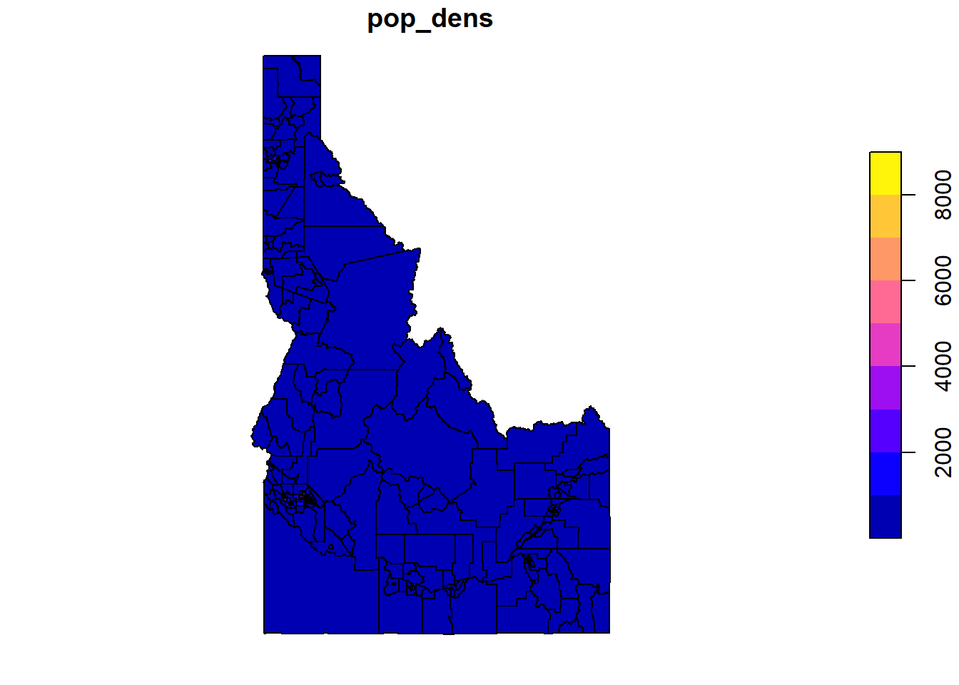

Code

library(tmap)

Breaking News: tmap 3.x is retiring. Please test v4, e.g. with
remotes::install_github('r-tmap/tmap')

Code

tm_shape(cejst_id_join) +
  tm_polygons(col = "pop_dens")

Code

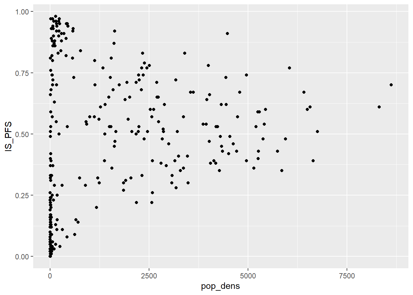
ggplot(cejst_id_join, aes(x=pop_dens, y=IS_PFS)) +
  geom_point()