Code
library(rgbif)
library(sf, quietly = TRUE)
library(spatstat, quietly = TRUE)
library(tidyverse, quietly = TRUE)Load libraries:
library(rgbif)
library(sf, quietly = TRUE)
library(spatstat, quietly = TRUE)
library(tidyverse, quietly = TRUE)Get data:
id <- tigris::states(progress_bar = FALSE) %>%
  filter(NAME == "Idaho") %>%
  st_transform(crs=4326)
Retrieving data for the year 2021gold_eag <- occ_search(scientificName = "Aquila chrysaetos",
country = "US",
hasCoordinate = TRUE,
limit = 1000)Prepare data for analysis:
gold_eag_dat <- gold_eag$data# convert to spatial data
gold_eag_sf <- gold_eag_dat %>%
filter(!is.na(decimalLatitude) & !is.na(decimalLongitude)) %>%
st_as_sf(., coords = c("decimalLongitude", "decimalLatitude"), crs=4326)
plot(st_geometry(gold_eag_sf))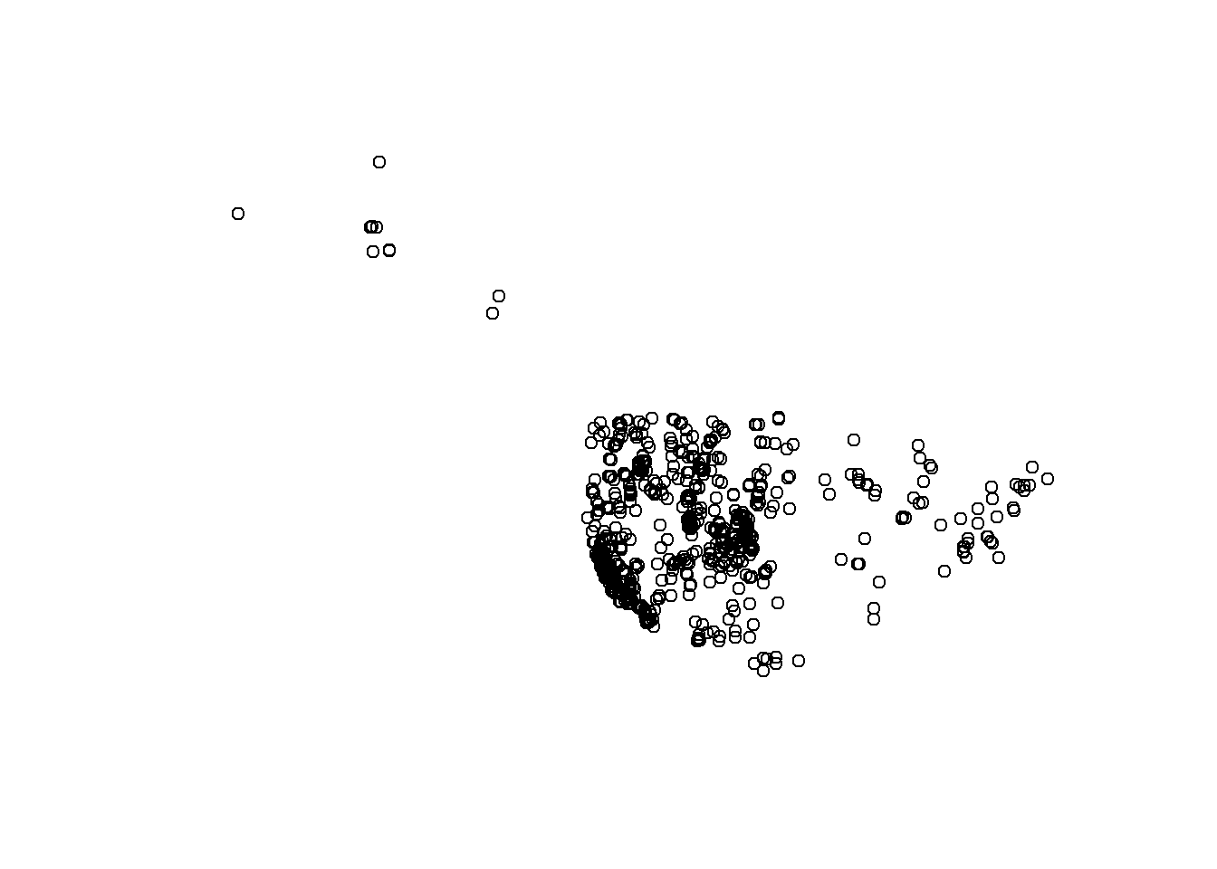
# subset to study area
gold_eag_id <- gold_eag_sf[id, ]

plot(st_geometry(id))
plot(st_geometry(gold_eag_id), add=TRUE)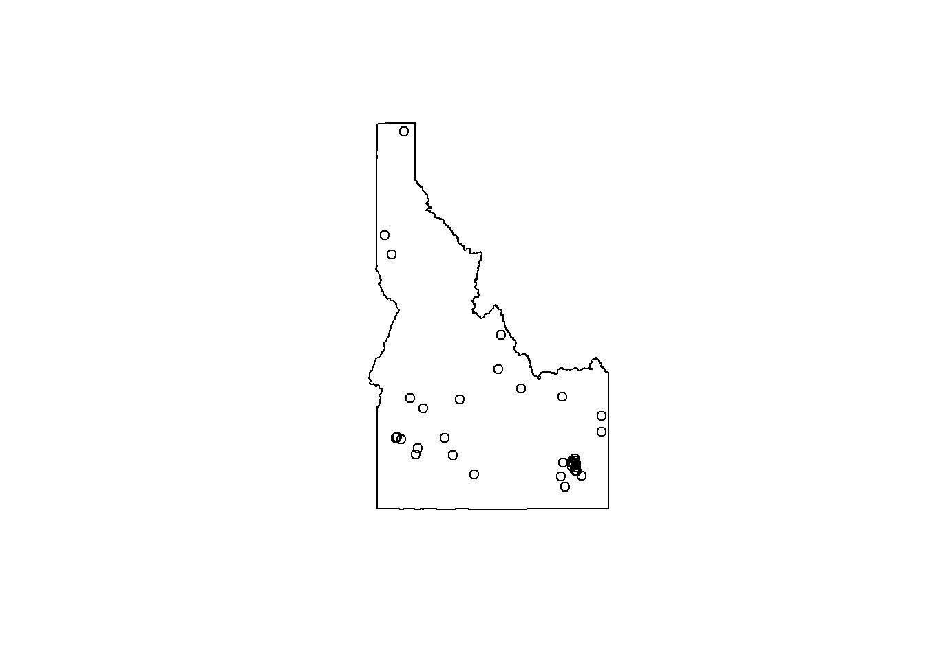
# must be mapped on a plane - projected CRS
gold_eag_id_proj <- st_transform(gold_eag_id, crs = 5070)
id_proj <- st_transform(id, crs = 5070)# convert to ppp object
gold_eag.ppp <- gold_eag_id_proj %>%
as.ppp()Warning in as.ppp.sf(.): only first attribute column is used for marks# remove marks from points
marks(gold_eag.ppp) <- NULL
# set study area to Idaho
Window(gold_eag.ppp) <- as.owin(id_proj)
plot(gold_eag.ppp)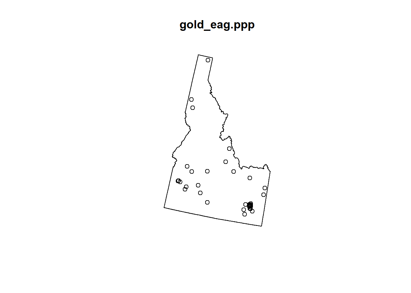
kde0 <- density(gold_eag.ppp)
plot(kde0, main="Default KDE for ID golden eagles")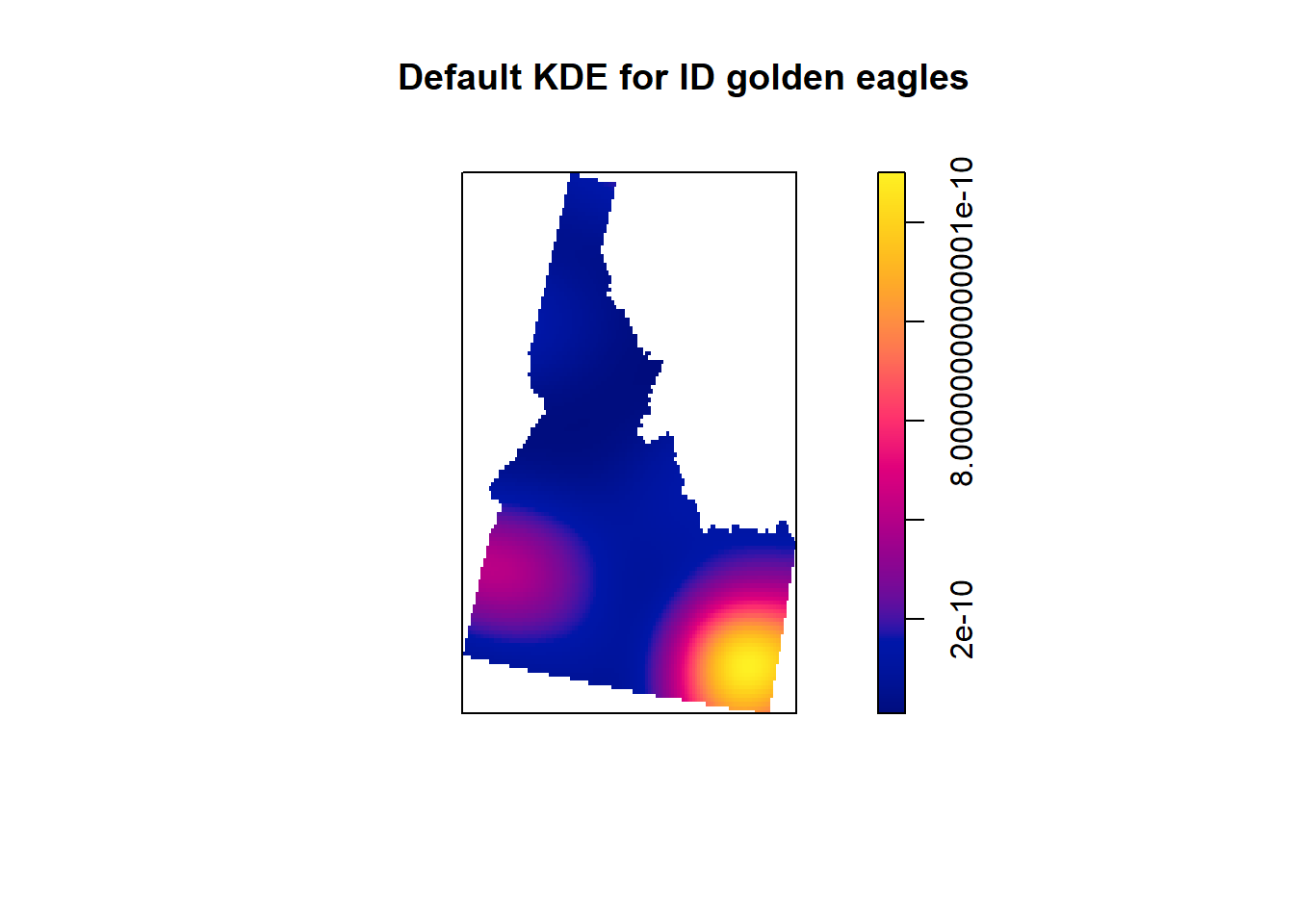
kde1 <- density(gold_eag.ppp, adjust = 0.75)
plot(kde1, main="Bandwidth reduced by 0.75")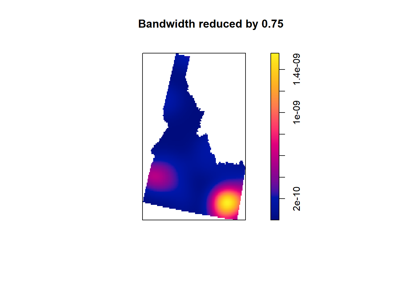
k0 <- Kest(gold_eag.ppp)
plot(k0)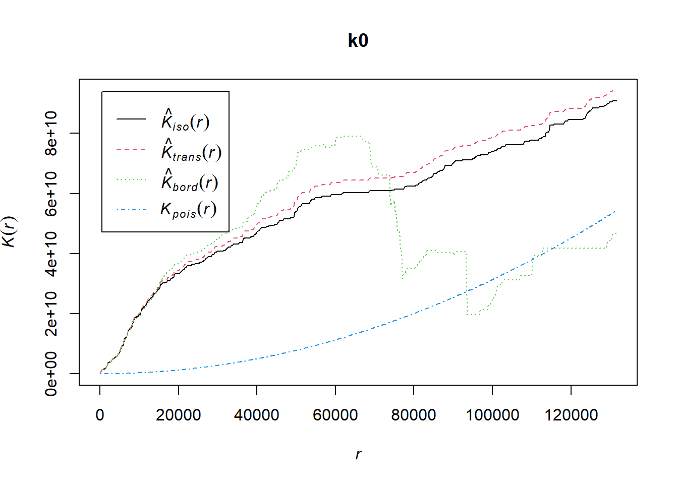
The x axis shows the increasing radius of the circle tested and the y axis shows the \(K\) at any given radius.
Different color lines show difference edge corrections. In the next step, we used border because it is the fastest. More information on edge correction can be found in the details section of the Kest help file (?Kest).
To test whether our points are clustered, we generate a \(K\) for completely spatially random points (red line below).
k.env <- envelope(gold_eag.ppp, correction="border", envelope = FALSE)Generating 99 simulations of CSR ...
1, 2, 3, 4, 5, 6, 7, 8, 9, 10, 11, 12, 13, 14, 15, 16, 17, 18, 19, 20,
21, 22, 23, 24, 25, 26, 27, 28, 29, 30, 31, 32, 33, 34, 35, 36, 37, 38, 39, 40,
41, 42, 43, 44, 45, 46, 47, 48, 49, 50, 51, 52, 53, 54, 55, 56, 57, 58, 59, 60,
61, 62, 63, 64, 65, 66, 67, 68, 69, 70, 71, 72, 73, 74, 75, 76, 77, 78, 79, 80,
81, 82, 83, 84, 85, 86, 87, 88, 89, 90, 91, 92, 93, 94, 95, 96, 97, 98,
99.
Done.plot(k.env)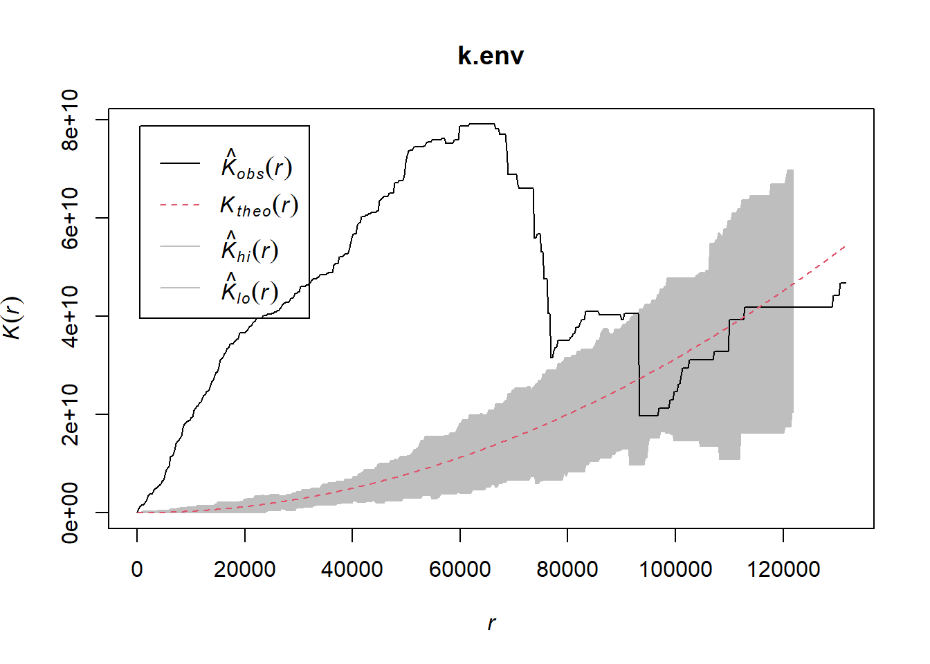
The error is generated by the 99 simulations of CSR referred to in the function printout. Here, we see our data are clustered (spatially autocorrelated) from the very smallest scale (r = 1) to a radius of about 90,000 meters.