Code
library(terra)
library(tmap)
library(sf)
library(tidyverse)
library(spatstat)  # Used for the dirichlet tesselation function
library(sp)Load libraries:
library(terra)
library(tmap)
library(sf)
library(tidyverse)
library(spatstat) # Used for the dirichlet tesselation function
library(sp)Get data:
aq <- read_csv("/opt/data/data/classexamples/ad_viz_plotval_data_PM25_2024_ID.csv") %>%
  st_as_sf(., coords = c("Site Longitude", "Site Latitude"), crs = "EPSG:4326") %>%
  st_transform(., crs = "EPSG:8826") %>%
  mutate(date = as_date(parse_datetime(Date, "%m/%d/%Y"))) %>%
  filter(., date >= 2024-07-01) %>%
  filter(., date > "2024-07-01" & date < "2024-07-31")
aq.sum <- aq %>%
  group_by(., `Site ID`) %>%
  summarise(., meanpm25 = mean(`Daily AQI Value`))

id.cty <- tigris::counties(state = "ID") %>%
st_transform(., crs = st_crs(aq.sum))#set up interpolation grid
# Create an empty grid where n is the total number of cells
grd <- st_make_grid(id.cty, n=150,
what = "centers") %>%
st_as_sf() %>%
mutate(X = st_coordinates(.)[, 1],
Y = st_coordinates(.)[, 2])
# Define the polynomial equation
f.0 <- as.formula(meanpm25 ~ 1)
# Run the regression model
lm.0 <- lm( f.0 , data=aq.sum)
# Use the regression model output to interpolate the surface
grd$var0.pred <- predict(lm.0, newdata = grd)
# Use data.frame without geometry to convert to raster
dat.0th <- grd %>%
select(X, Y, var0.pred) %>%
st_drop_geometry()
# Convert to raster object to take advantage of rasterVis' imaging
# environment
r <- rast(dat.0th, crs = crs(grd))
r.m <- mask(r, st_as_sf(id.cty))
tm_shape(r.m) +
tm_raster( title="Predicted air quality") +
tm_shape(aq.sum) +
tm_dots(size=0.2) +
tm_legend(legend.outside=TRUE)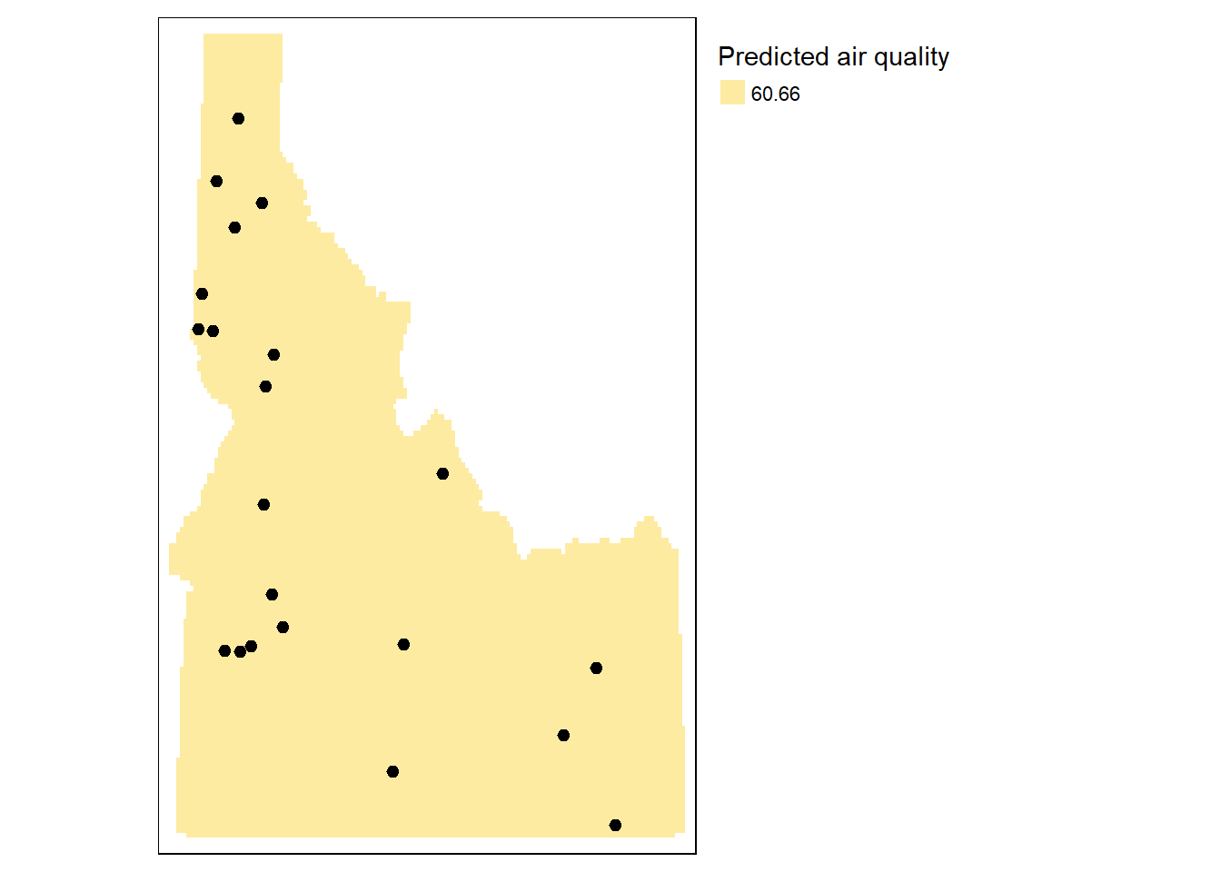
# Define the polynomial equation
f.1  <- as.formula(meanpm25 ~ X + Y)

aq.sum$X <- st_coordinates(aq.sum)[,1]
aq.sum$Y <- st_coordinates(aq.sum)[,2]

# Run the regression model
lm.1 <- lm( f.1 , data=aq.sum)

# Use the regression model output to interpolate the surface
grd$var1.pred <- predict(lm.1, newdata = grd)
# Use data.frame without geometry to convert to raster
dat.1st <- grd %>%
  select(X, Y, var1.pred) %>%
  st_drop_geometry()

# Convert to raster object to take advantage of rasterVis' imaging
# environment
r   <- rast(dat.1st, crs = crs(grd))
r.m <- mask(r, st_as_sf(id.cty))

tm_shape(r.m) +
  tm_raster( title="Predicted air quality") +
  tm_shape(aq.sum) +
  tm_dots(size=0.2) +
  tm_legend(legend.outside=TRUE)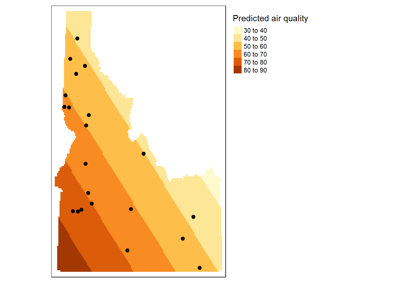
# Define the 1st order polynomial equation
f.2 <- as.formula(meanpm25 ~ X + Y + I(X*X)+I(Y*Y) + I(X*Y))

# Run the regression model
lm.2 <- lm( f.2, data=aq.sum)

# Use the regression model output to interpolate the surface
grd$var2.pred <- predict(lm.2, newdata = grd)
# Use data.frame without geometry to convert to raster
dat.2nd <- grd %>%
  select(X, Y, var2.pred) %>%
  st_drop_geometry()

r   <- rast(dat.2nd, crs = crs(grd))
r.m <- mask(r, st_as_sf(id.cty))

tm_shape(r.m) + tm_raster(n=10, title="Predicted air quality") +
  tm_shape(aq.sum) +
  tm_dots(size=0.2) +
  tm_legend(legend.outside=TRUE)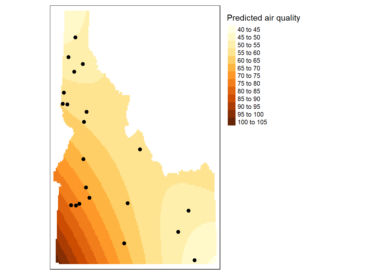
aq.sum$res <- lm.2$residualsvar.cld <- gstat::variogram(res ~ 1, aq.sum, cloud = TRUE)
var.df <- as.data.frame(var.cld)
index1 <- which(with(var.df, left==21 & right==2))
OP <- par( mar=c(4,6,1,1))
plot(var.cld$dist/1000 , var.cld$gamma, col="grey",
xlab = "Distance between point pairs (km)",
ylab = expression( frac((res[2] - res[1])^2 , 2)) )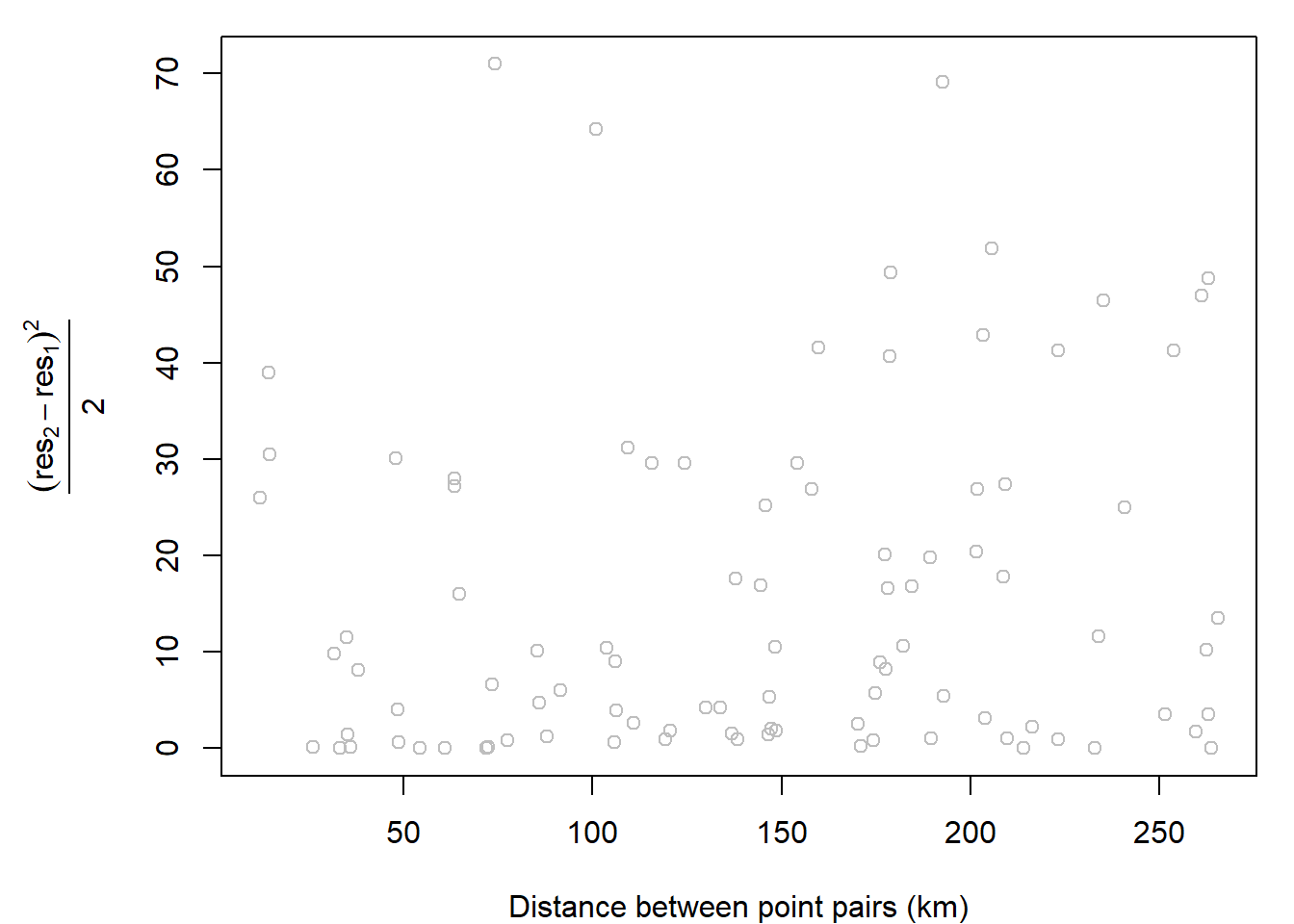
# Compute the sample variogram, note the f.2 trend model is one of the parameters
# passed to variogram(). This tells the function to create the variogram on
# the de-trended data
var.smpl <- gstat::variogram(f.2, aq.sum, cloud = FALSE, cutoff = 1000000, width = 89900)


# Compute the variogram model by passing the nugget, sill and range values
# to fit.variogram() via the vgm() function.
dat.fit  <- gstat::fit.variogram(var.smpl, gstat::vgm(nugget = 12, range= 60000, model="Gau", cutoff=1000000))
Warning in gstat::fit.variogram(var.smpl, gstat::vgm(nugget = 12, range =
60000, : No convergence after 200 iterations: try different initial values?# The following plot allows us to gauge the fit
plot(var.smpl, dat.fit)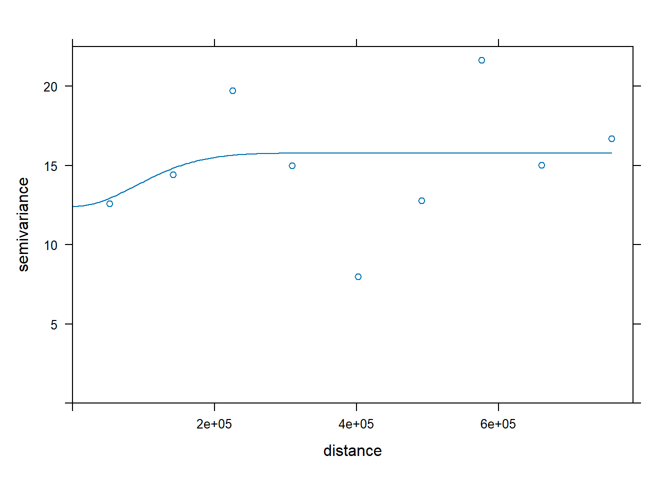
dat.krg <- gstat::krige( formula = f.2,
locations = aq.sum,
newdata = grd[, c("X", "Y", "var2.pred")],
model = dat.fit)[using universal kriging]dat.krg.preds <- dat.krg %>%
mutate(X = st_coordinates(.)[, 1],
Y = st_coordinates(.)[, 2]) %>%
select(X, Y, var1.pred) %>%
st_drop_geometry()
dat.krg.var <- dat.krg %>%
mutate(X = st_coordinates(.)[, 1],
Y = st_coordinates(.)[, 2]) %>%
select(X, Y, var1.var) %>%
st_drop_geometry()
r <- rast(dat.krg.preds, crs = crs(grd))
r.m <- mask(r, st_as_sf(id.cty))
r.var <- rast(dat.krg.var, crs = crs(grd))
r.m.var <- mask(r.var, st_as_sf(id.cty))
# Plot the raster and the sampled points
tm_shape(r.m) + tm_raster(n=10, title="Predicted air quality") +tm_shape(aq.sum) + tm_dots(size=0.2) +
tm_legend(legend.outside=TRUE)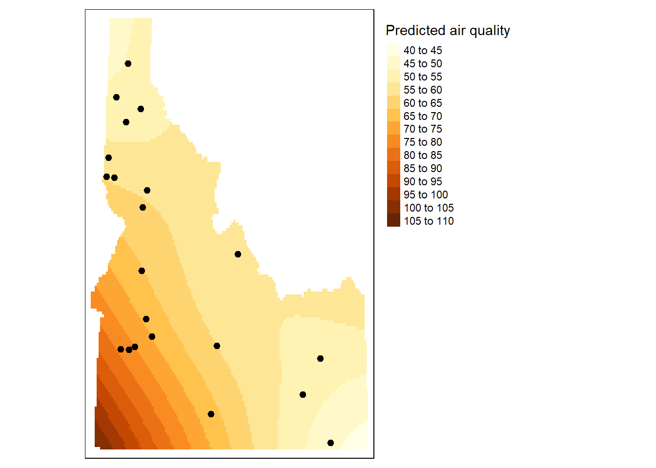
We tried changing the model, nugget, range, and psill arguments in gstat::vgm.
# Compute the sample variogram, note the f.2 trend model is one of the parameters
# passed to variogram(). This tells the function to create the variogram on
# the de-trended data
var.smpl <- gstat::variogram(f.2, aq.sum, cloud = FALSE, cutoff = 1000000, width = 89900)
# Compute the variogram model by passing the nugget, sill and range values
# to fit.variogram() via the vgm() function.
dat.fit <- gstat::fit.variogram(var.smpl, gstat::vgm(model="Sph",
nugget = 10,
range = 60000))
# The following plot allows us to gauge the fit
plot(var.smpl, dat.fit)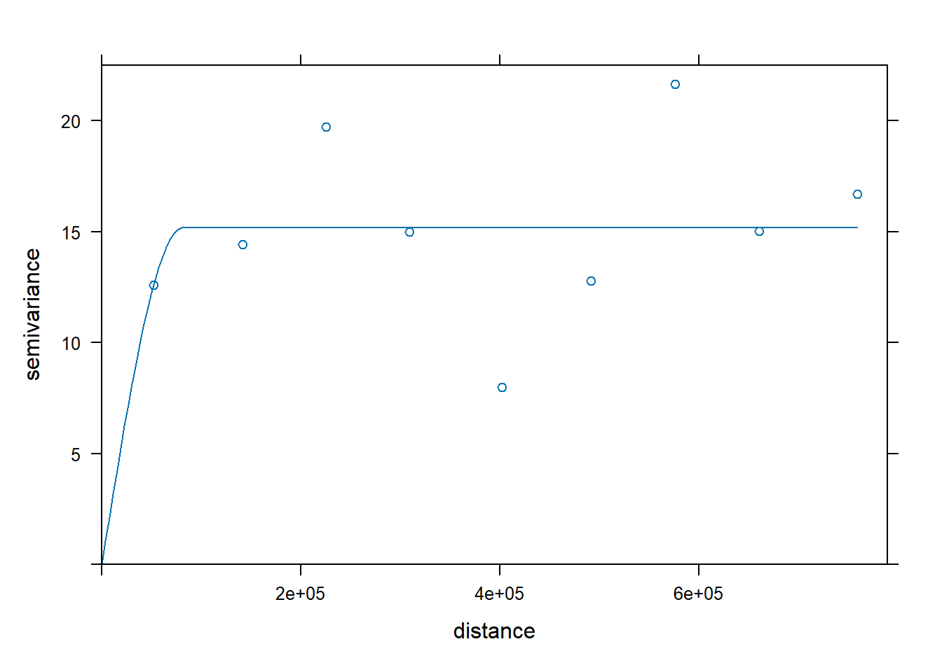
dat.krg <- gstat::krige( formula = f.2,
                         locations = aq.sum,
                         newdata = grd[, c("X", "Y", "var2.pred")],
                         model = dat.fit)
[using universal kriging]dat.krg.preds <- dat.krg %>%
mutate(X = st_coordinates(.)[, 1],
Y = st_coordinates(.)[, 2]) %>%
select(X, Y, var1.pred) %>%
st_drop_geometry()
dat.krg.var <- dat.krg %>%
mutate(X = st_coordinates(.)[, 1],
Y = st_coordinates(.)[, 2]) %>%
select(X, Y, var1.var) %>%
st_drop_geometry()
r <- rast(dat.krg.preds, crs = crs(grd))
r.m <- mask(r, st_as_sf(id.cty))
r.var <- rast(dat.krg.var, crs = crs(grd))
r.m.var <- mask(r.var, st_as_sf(id.cty))
# Plot the raster and the sampled points
tm_shape(r.m) + tm_raster(n=10, title="Predicted air quality") +tm_shape(aq.sum) + tm_dots(size=0.2) +
tm_legend(legend.outside=TRUE)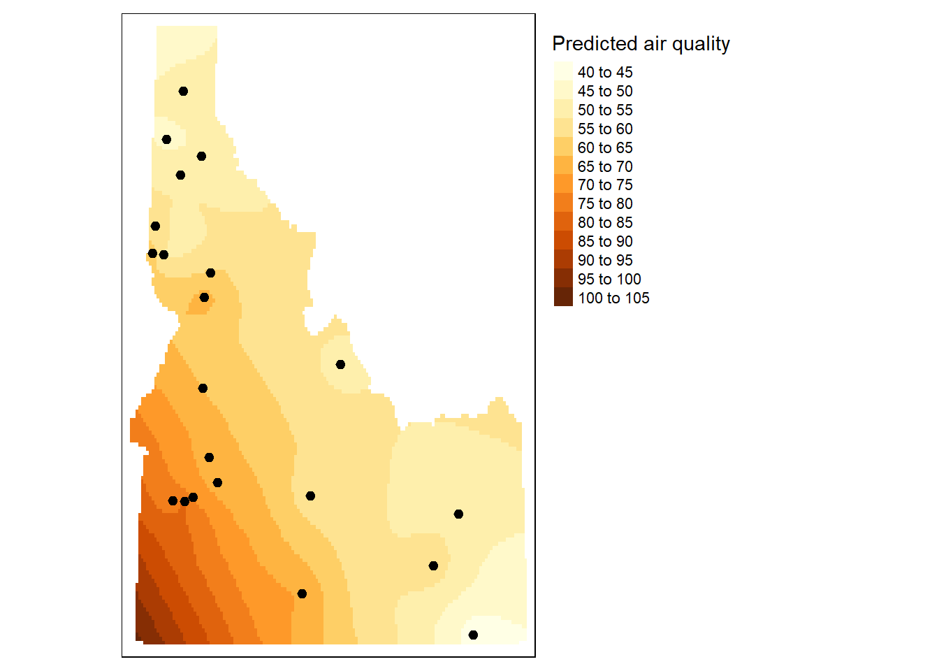
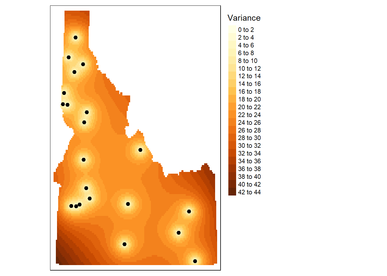
tm_shape(r.m.var) + tm_raster(n=20, title="Variance") +tm_shape(aq.sum) + tm_dots(size=0.2) +
  tm_legend(legend.outside=TRUE)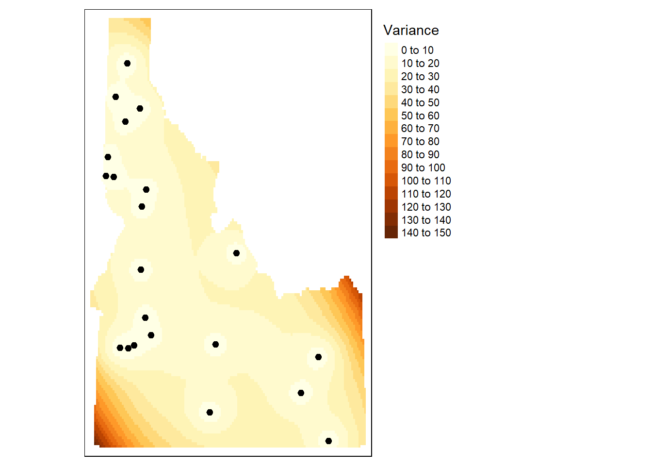
# Compute the sample variogram, note the f.2 trend model is one of the parameters
# passed to variogram(). This tells the function to create the variogram on
# the de-trended data
var.smpl <- gstat::variogram(f.1, aq.sum, cloud = FALSE, cutoff = 1000000, width = 89900)


# Compute the variogram model by passing the nugget, sill and range values
# to fit.variogram() via the vgm() function.
dat.fit  <- gstat::fit.variogram(var.smpl, gstat::vgm(model="Exp",
                                                      nugget = 20))
Warning in gstat::fit.variogram(var.smpl, gstat::vgm(model = "Exp", nugget =
20)): No convergence after 200 iterations: try different initial values?# The following plot allows us to gauge the fit
plot(var.smpl, dat.fit)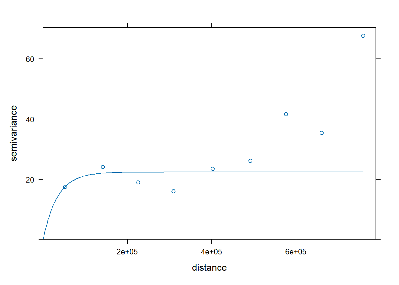
dat.krg <- gstat::krige( formula = f.1,
                         locations = aq.sum,
                         newdata = grd[, c("X", "Y", "var1.pred")],
                         model = dat.fit)
[using universal kriging]dat.krg.preds <- dat.krg %>%
mutate(X = st_coordinates(.)[, 1],
Y = st_coordinates(.)[, 2]) %>%
select(X, Y, var1.pred) %>%
st_drop_geometry()
dat.krg.var <- dat.krg %>%
mutate(X = st_coordinates(.)[, 1],
Y = st_coordinates(.)[, 2]) %>%
select(X, Y, var1.var) %>%
st_drop_geometry()
r <- rast(dat.krg.preds, crs = crs(grd))
r.m <- mask(r, st_as_sf(id.cty))
r.var <- rast(dat.krg.var, crs = crs(grd))
r.m.var <- mask(r.var, st_as_sf(id.cty))
# Plot the raster and the sampled points
tm_shape(r.m) + tm_raster(n=10, title="Predicted air quality") +tm_shape(aq.sum) + tm_dots(size=0.2) +
tm_legend(legend.outside=TRUE)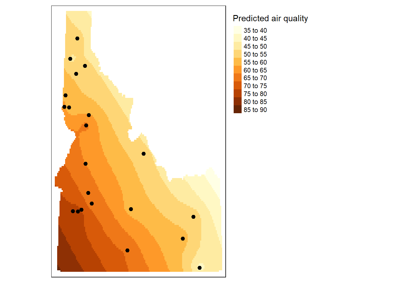
tm_shape(r.m.var) + tm_raster(n=20, title="Variance") +tm_shape(aq.sum) + tm_dots(size=0.2) +
  tm_legend(legend.outside=TRUE)