Session 16 code

Author

Carolyn Koehn

Load libraries:

Code

library(tidyverse)
library(sf)
library(terra)

Load data:

Code

hospitals_pnw <- read_csv("/opt/data/data/assignment06/landmarks_pnw.csv") %>%
  filter(., MTFCC == "K2543") %>%
  st_as_sf(., coords = c("longitude", "latitude"), crs=4269) %>%
  st_transform(crs = 5070)

Rasterize

Code

raster_template = rast(ext(hospitals_pnw), resolution = 10000,
                       crs = st_crs(hospitals_pnw)$wkt)

hosp_raster1 = rasterize(hospitals_pnw, raster_template,
                         field = 1)

plot(hosp_raster1, colNA = "navy")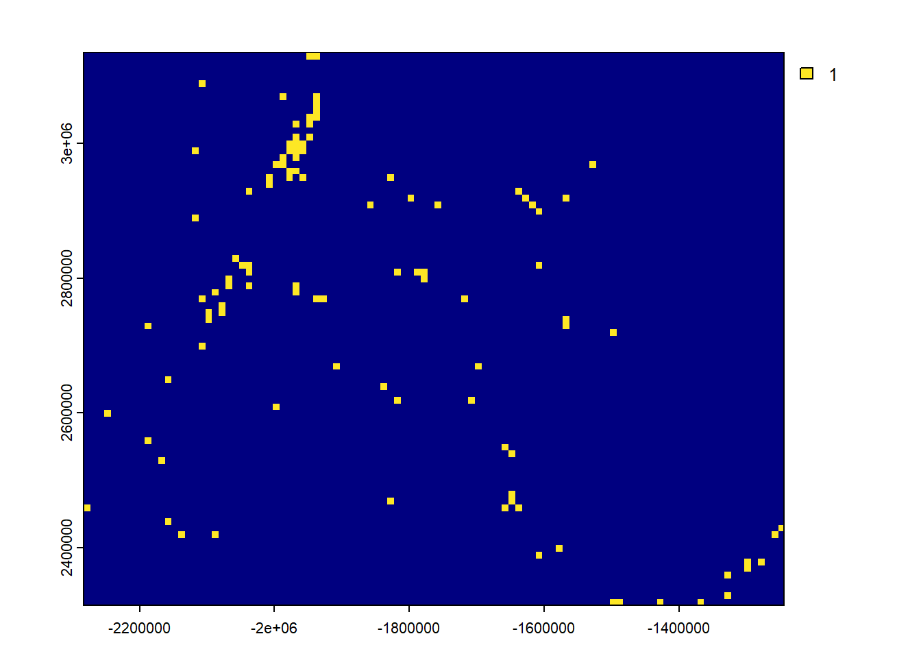

Code

# add dummy numeric data
hospitals_pnw$rand_capacity <- rnorm(n = nrow(hospitals_pnw),
                                     mean = 5000,
                                     sd = 2000)

hosp_raster3 = rasterize(hospitals_pnw, raster_template, 
                         field = "rand_capacity", fun = sum)

plot(hosp_raster3)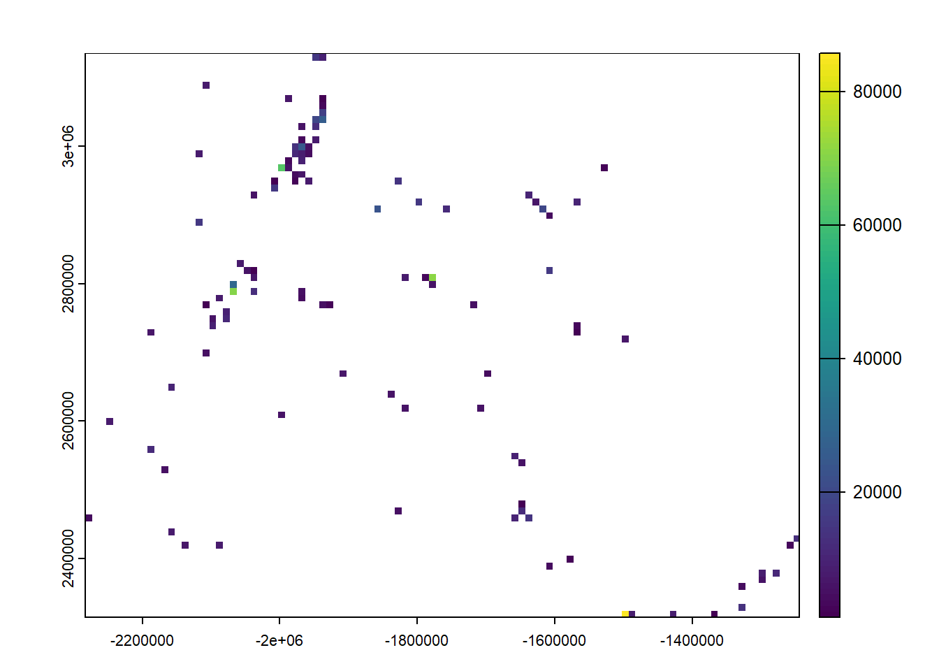

Raster to Vector

Code

dem = rast(system.file("raster/dem.tif", package = "spDataLarge"))
cl = as.contour(dem)

Creating New Data

Distance

Code

raster_template = rast(ext(hospitals_pnw), resolution = 1000,
                       crs = st_crs(hospitals_pnw)$wkt)
hosp_raster1 = rasterize(hospitals_pnw, raster_template,
                       field = 1)

hosp_dist_rast <- distance(hosp_raster1)
plot(hosp_dist_rast)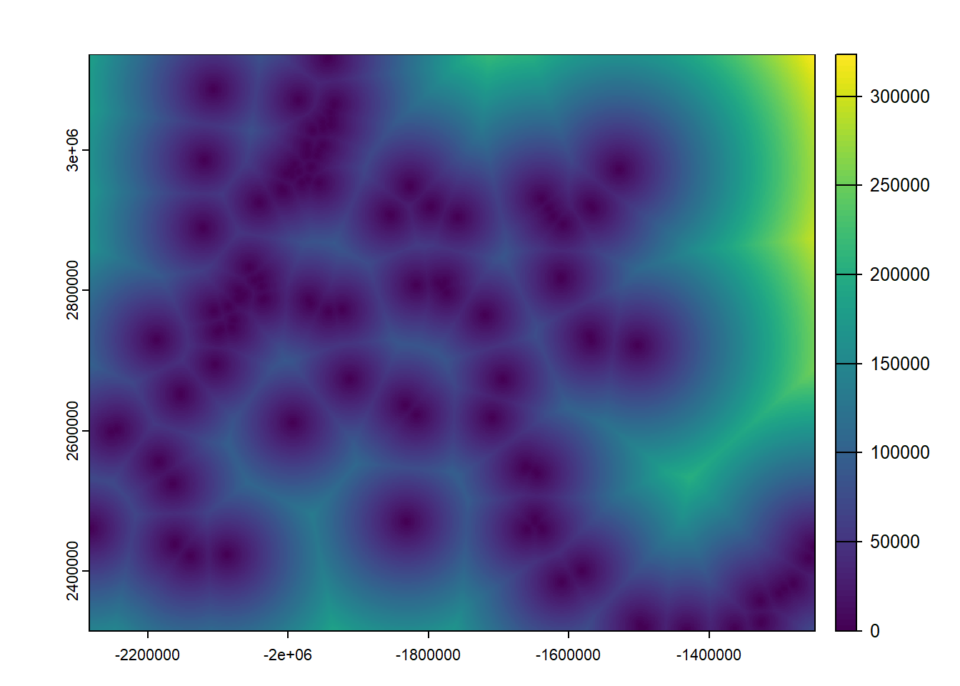

Attributes

Code

wildfire_haz <- rast("/opt/data/data/assignment07/wildfire_hazard_agg.tif")

Code

hospitals_pnw_proj <- st_transform(hospitals_pnw, crs(wildfire_haz))

hosp_fire_haz <- terra::extract(wildfire_haz, hospitals_pnw_proj)
head(hosp_fire_haz)

  ID    WHP_ID
1  1 1952.8750
2  2    0.0000
3  3  741.4531
4  4  200.2812
5  5    0.0000
6  6  150.5938

Code

hospitals_pnw_proj$wildfire <- hosp_fire_haz$WHP_ID

Code

cejst <- st_read("/opt/data/data/assignment06/cejst_pnw.shp") %>%
  st_transform(crs = crs(wildfire_haz)) %>%
  filter(!st_is_empty(.))

Code

wildfire.zones <- terra::zonal(wildfire_haz, vect(cejst), fun="mean", na.rm=TRUE)

head(wildfire.zones)

       WHP_ID
1    3.053172
2 2997.795051
3    6.647930
4   85.971309
5   34.706535
6   17.306250

Practice

Step 1: Load libraries

Code

library(sf)
library(terra)
library(tidyverse)
library(tmap)

Step 2: Load in data

We loaded the wildfire hazard data and the cejst data earlier in the example.

Code

# custom function to download and load Forest Service data
download_unzip_read <- function(link){
  tmp <- tempfile()
  download.file(link, tmp)
  tmp2 <- tempfile()
  unzip(zipfile=tmp, exdir=tmp2)
  shapefile.sf <- read_sf(tmp2)
}

### FS Boundaries
fs.url <- "https://data.fs.usda.gov/geodata/edw/edw_resources/shp/S_USA.AdministrativeForest.zip"
fs.bdry <- download_unzip_read(link = fs.url)

### CFLRP Data
cflrp.url <- "https://data.fs.usda.gov/geodata/edw/edw_resources/shp/S_USA.CFLR_HPRP_ProjectBoundary.zip"
cflrp.bdry <- download_unzip_read(link = cflrp.url)

Step 3: Check validity

Code

all(st_is_valid(fs.bdry))

[1] FALSE

Code

all(st_is_valid(cflrp.bdry))

[1] FALSE

Code

fs.bdry <- st_make_valid(fs.bdry)

cflrp.bdry <- st_make_valid(cflrp.bdry)

Code

all(st_is_valid(fs.bdry))

[1] TRUE

Code

all(st_is_valid(cflrp.bdry))

[1] TRUE

Step 3: Check alignment

Code

st_crs(fs.bdry)

Coordinate Reference System:
  User input: NAD83 
  wkt:
GEOGCRS["NAD83",
    DATUM["North American Datum 1983",
        ELLIPSOID["GRS 1980",6378137,298.257222101,
            LENGTHUNIT["metre",1]]],
    PRIMEM["Greenwich",0,
        ANGLEUNIT["degree",0.0174532925199433]],
    CS[ellipsoidal,2],
        AXIS["latitude",north,
            ORDER[1],
            ANGLEUNIT["degree",0.0174532925199433]],
        AXIS["longitude",east,
            ORDER[2],
            ANGLEUNIT["degree",0.0174532925199433]],
    ID["EPSG",4269]]

Code

st_crs(wildfire_haz)

Coordinate Reference System:
  User input: unnamed 
  wkt:
PROJCRS["unnamed",
    BASEGEOGCRS["NAD83",
        DATUM["North American Datum 1983",
            ELLIPSOID["GRS 1980",6378137,298.257222101004,
                LENGTHUNIT["metre",1]]],
        PRIMEM["Greenwich",0,
            ANGLEUNIT["degree",0.0174532925199433]],
        ID["EPSG",4269]],
    CONVERSION["Albers Equal Area",
        METHOD["Albers Equal Area",
            ID["EPSG",9822]],
        PARAMETER["Latitude of false origin",23,
            ANGLEUNIT["degree",0.0174532925199433],
            ID["EPSG",8821]],
        PARAMETER["Longitude of false origin",-96,
            ANGLEUNIT["degree",0.0174532925199433],
            ID["EPSG",8822]],
        PARAMETER["Latitude of 1st standard parallel",29.5,
            ANGLEUNIT["degree",0.0174532925199433],
            ID["EPSG",8823]],
        PARAMETER["Latitude of 2nd standard parallel",45.5,
            ANGLEUNIT["degree",0.0174532925199433],
            ID["EPSG",8824]],
        PARAMETER["Easting at false origin",0,
            LENGTHUNIT["metre",1],
            ID["EPSG",8826]],
        PARAMETER["Northing at false origin",0,
            LENGTHUNIT["metre",1],
            ID["EPSG",8827]]],
    CS[Cartesian,2],
        AXIS["easting",east,
            ORDER[1],
            LENGTHUNIT["metre",1,
                ID["EPSG",9001]]],
        AXIS["northing",north,
            ORDER[2],
            LENGTHUNIT["metre",1,
                ID["EPSG",9001]]]]

Code

st_crs(cflrp.bdry)

Coordinate Reference System:
  User input: NAD83 
  wkt:
GEOGCRS["NAD83",
    DATUM["North American Datum 1983",
        ELLIPSOID["GRS 1980",6378137,298.257222101,
            LENGTHUNIT["metre",1]]],
    PRIMEM["Greenwich",0,
        ANGLEUNIT["degree",0.0174532925199433]],
    CS[ellipsoidal,2],
        AXIS["latitude",north,
            ORDER[1],
            ANGLEUNIT["degree",0.0174532925199433]],
        AXIS["longitude",east,
            ORDER[2],
            ANGLEUNIT["degree",0.0174532925199433]],
    ID["EPSG",4269]]

Code

st_crs(cejst)

Coordinate Reference System:
  User input: PROJCRS["unnamed",
    BASEGEOGCRS["NAD83",
        DATUM["North American Datum 1983",
            ELLIPSOID["GRS 1980",6378137,298.257222101004,
                LENGTHUNIT["metre",1]]],
        PRIMEM["Greenwich",0,
            ANGLEUNIT["degree",0.0174532925199433]],
        ID["EPSG",4269]],
    CONVERSION["Albers Equal Area",
        METHOD["Albers Equal Area",
            ID["EPSG",9822]],
        PARAMETER["Latitude of false origin",23,
            ANGLEUNIT["degree",0.0174532925199433],
            ID["EPSG",8821]],
        PARAMETER["Longitude of false origin",-96,
            ANGLEUNIT["degree",0.0174532925199433],
            ID["EPSG",8822]],
        PARAMETER["Latitude of 1st standard parallel",29.5,
            ANGLEUNIT["degree",0.0174532925199433],
            ID["EPSG",8823]],
        PARAMETER["Latitude of 2nd standard parallel",45.5,
            ANGLEUNIT["degree",0.0174532925199433],
            ID["EPSG",8824]],
        PARAMETER["Easting at false origin",0,
            LENGTHUNIT["metre",1],
            ID["EPSG",8826]],
        PARAMETER["Northing at false origin",0,
            LENGTHUNIT["metre",1],
            ID["EPSG",8827]]],
    CS[Cartesian,2],
        AXIS["easting",east,
            ORDER[1],
            LENGTHUNIT["metre",1,
                ID["EPSG",9001]]],
        AXIS["northing",north,
            ORDER[2],
            LENGTHUNIT["metre",1,
                ID["EPSG",9001]]]] 
  wkt:
PROJCRS["unnamed",
    BASEGEOGCRS["NAD83",
        DATUM["North American Datum 1983",
            ELLIPSOID["GRS 1980",6378137,298.257222101004,
                LENGTHUNIT["metre",1]]],
        PRIMEM["Greenwich",0,
            ANGLEUNIT["degree",0.0174532925199433]],
        ID["EPSG",4269]],
    CONVERSION["Albers Equal Area",
        METHOD["Albers Equal Area",
            ID["EPSG",9822]],
        PARAMETER["Latitude of false origin",23,
            ANGLEUNIT["degree",0.0174532925199433],
            ID["EPSG",8821]],
        PARAMETER["Longitude of false origin",-96,
            ANGLEUNIT["degree",0.0174532925199433],
            ID["EPSG",8822]],
        PARAMETER["Latitude of 1st standard parallel",29.5,
            ANGLEUNIT["degree",0.0174532925199433],
            ID["EPSG",8823]],
        PARAMETER["Latitude of 2nd standard parallel",45.5,
            ANGLEUNIT["degree",0.0174532925199433],
            ID["EPSG",8824]],
        PARAMETER["Easting at false origin",0,
            LENGTHUNIT["metre",1],
            ID["EPSG",8826]],
        PARAMETER["Northing at false origin",0,
            LENGTHUNIT["metre",1],
            ID["EPSG",8827]]],
    CS[Cartesian,2],
        AXIS["easting",east,
            ORDER[1],
            LENGTHUNIT["metre",1,
                ID["EPSG",9001]]],
        AXIS["northing",north,
            ORDER[2],
            LENGTHUNIT["metre",1,
                ID["EPSG",9001]]]]

Code

st_crs(wildfire_haz) == st_crs(cejst)

[1] TRUE

Code

st_crs(wildfire_haz) == st_crs(fs.bdry)

[1] FALSE

Code

target_crs <- st_crs(wildfire_haz)

Code

fs.bdry_proj <- st_transform(fs.bdry, crs = target_crs)
st_crs(fs.bdry_proj) == target_crs

[1] TRUE

Code

st_crs(fs.bdry_proj) == st_crs(wildfire_haz)

[1] TRUE

Code

cflrp.bdry_proj <- st_transform(cflrp.bdry, crs = st_crs(wildfire_haz))

Step 4: Subset to geographies

cejst is our study area (the Pacific Northwest) to subset to.

Code

fs.subset <- fs.bdry_proj[cejst, ]
cflrp.subset <- cflrp.bdry_proj[cejst, ]

# keep only tracts that intersect Forest Service land
cejst.subset <- cejst[fs.subset, ]

Step 5: Select attributes of interest

Code

cejst.df <- cejst.subset %>% 
  select(GEOID10, LMI_PFS, LHE, HBF_PFS)
head(cejst.df)

Simple feature collection with 6 features and 4 fields
Geometry type: MULTIPOLYGON
Dimension:     XY
Bounding box:  xmin: -1598729 ymin: 2388182 xmax: -1475201 ymax: 3000813
Projected CRS: unnamed
       GEOID10 LMI_PFS LHE HBF_PFS                       geometry
2  16025970100    0.75   0    0.60 MULTIPOLYGON (((-1485848 24...
17 16057005500    0.43   0    0.44 MULTIPOLYGON (((-1567845 28...
21 16057005600    0.30   0    0.05 MULTIPOLYGON (((-1573408 28...
22 16009950100    0.55   1    0.40 MULTIPOLYGON (((-1566013 28...
23 16017950500    0.75   1    0.53 MULTIPOLYGON (((-1545064 29...
24 16017950400    0.60   1    0.68 MULTIPOLYGON (((-1544958 29...

Step 6: Extract wildfire hazard

Code

cejst.fire <- terra::extract(wildfire_haz, vect(cejst.df), fun=mean, na.rm=TRUE)
head(cejst.fire)

  ID    WHP_ID
1  1 2997.7951
2  2  182.8864
3  3  386.9580
4  4  173.1703
5  5  193.4199
6  6  210.4406

Code

cejst.df$WHP_ID <- cejst.fire$WHP_ID

Step 7: Does each tract intersect a CFLRP boundary?

Code

cejst.cflrp <- apply(st_intersects(cejst.df, cflrp.subset, sparse=FALSE), 1, any)

Code

cejst.df <- cejst.df %>%
  mutate(CFLRP = cejst.cflrp)

Step 8: Compare areas

Many comparisons are possible! Here are some examples.

Code

cflrp.summ <- cejst.df %>%
  st_drop_geometry() %>%
  group_by(CFLRP) %>%
  summarise(across(LMI_PFS:WHP_ID, ~ mean(.x, na.rm=TRUE)))

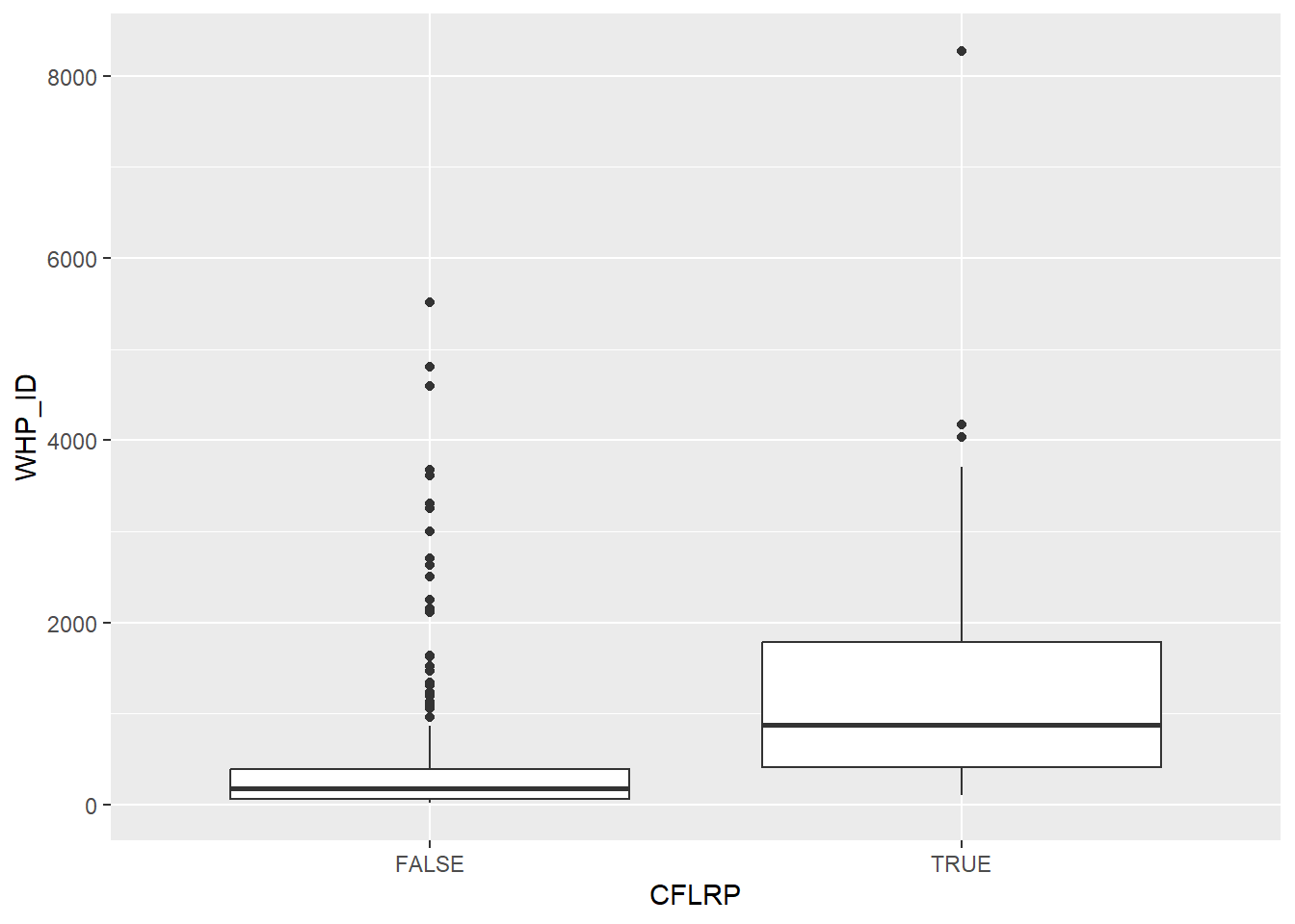
ggplot(data = cejst.df, aes(x=CFLRP, y=WHP_ID)) +
  geom_boxplot()