Session 23 code

Author

Carolyn Koehn

Code from last class

Pre-processing

Load libraries:

Code

library(sf)
library(terra)
library(tidyverse)
library(tmap)
library(tree)
library(randomForest)

Load data:

Code

download_unzip_read <- function(link){
  tmp <- tempfile()
  download.file(link, tmp)
  tmp2 <- tempfile()
  unzip(zipfile=tmp, exdir=tmp2)
  shapefile.sf <- read_sf(tmp2)
}

### FS Boundaries
fs.url <- "https://data.fs.usda.gov/geodata/edw/edw_resources/shp/S_USA.AdministrativeForest.zip"
fs.bdry <- download_unzip_read(link = fs.url)

### CFLRP Data
cflrp.url <- "https://data.fs.usda.gov/geodata/edw/edw_resources/shp/S_USA.CFLR_HPRP_ProjectBoundary.zip"
cflrp.bdry <- download_unzip_read(link = cflrp.url)

wildfire_haz <- rast("/opt/data/data/assignment01/wildfire_hazard_agg.tif")

cejst <- st_read("/opt/data/data/assignment01/cejst_nw.shp", quiet=TRUE) %>%
  filter(!st_is_empty(.))

Check validity:

Code

all(st_is_valid(fs.bdry))

[1] FALSE

Code

all(st_is_valid(cflrp.bdry))

[1] FALSE

Code

fs.bdry <- st_make_valid(fs.bdry)
cflrp.bdry <- st_make_valid(cflrp.bdry)

Check alignment:

Code

st_crs(wildfire_haz) == st_crs(fs.bdry)

[1] FALSE

Code

st_crs(wildfire_haz) == st_crs(cflrp.bdry)

[1] FALSE

Code

st_crs(wildfire_haz) == st_crs(cejst)

[1] FALSE

Code

fs.bdry_proj <- st_transform(fs.bdry, crs = st_crs(wildfire_haz))
cflrp.bdry_proj <- st_transform(cflrp.bdry, crs = st_crs(wildfire_haz))
cejst_proj <- st_transform(cejst, crs = st_crs(wildfire_haz))

Subset to relevant geographies:

Code

fs.bdry_sub <- fs.bdry_proj[cejst_proj, ]
cflrp.bdry_sub <- cflrp.bdry_proj[cejst_proj, ]

cejst_sub <- cejst_proj[fs.bdry_sub, ]

Select relevant attributes:

Code

cejst_sub <- cejst_sub %>%
  select(GEOID10, LMI_PFS, LHE, HBF_PFS)

Extract wildfire risk:

Code

wf_risk <- terra::extract(wildfire_haz, cejst_sub, fun=mean)

cejst_sub$WHP_ID <- wf_risk$WHP_ID

CFLRP T or F:

Code

cflrp <- apply(st_intersects(cejst_sub, cflrp.bdry_sub, sparse = FALSE), 1, any)

cejst_sub$CFLRP <- cflrp

Compare (three models)

Code

cejst_mod <- cejst_sub %>%
  st_drop_geometry(.) %>%
  na.omit(.)

cejst_mod[, c("LMI_PFS", "LHE", "HBF_PFS", "WHP_ID")] <- scale(cejst_mod[, c("LMI_PFS", "LHE", "HBF_PFS", "WHP_ID")])

Logistic regression:

Code

logistic.global <- glm(CFLRP ~ LMI_PFS + LHE + HBF_PFS + WHP_ID,
                       family = binomial(link = "logit"),
                       data = cejst_mod)
summary(logistic.global)


Call:
glm(formula = CFLRP ~ LMI_PFS + LHE + HBF_PFS + WHP_ID, family = binomial(link = "logit"), 
    data = cejst_mod)

Coefficients:
            Estimate Std. Error z value Pr(>|z|)    
(Intercept) -0.66462    0.14347  -4.632 3.62e-06 ***
LMI_PFS      0.17284    0.16881   1.024    0.306    
LHE         -0.25551    0.15791  -1.618    0.106    
HBF_PFS     -0.01511    0.16081  -0.094    0.925    
WHP_ID       0.88902    0.16785   5.297 1.18e-07 ***
---
Signif. codes:  0 '***' 0.001 '**' 0.01 '*' 0.05 '.' 0.1 ' ' 1

(Dispersion parameter for binomial family taken to be 1)

    Null deviance: 330.74  on 255  degrees of freedom
Residual deviance: 290.03  on 251  degrees of freedom
AIC: 300.03

Number of Fisher Scoring iterations: 4

Tree Model

Code

library(tree)
cejst_mod$CFLRP <- as.factor(ifelse(cejst_mod$CFLRP == 1, "Yes", "No"))
tree.model <- tree(CFLRP ~ LMI_PFS + LHE + HBF_PFS + WHP_ID, cejst_mod)

Random Forest

Code

library(randomForest)
class.model <- CFLRP ~ .
rf2 <- randomForest(formula = class.model, cejst_mod[,-1])

Model Comparison

Create train/test split

Code

# controls which random number generator is used so that my outputs will be consistent
# use a different one than me and see how our results differ!
set.seed(444)

library(caret)

Loading required package: lattice


Attaching package: 'caret'

The following object is masked from 'package:purrr':

    lift

Code

# get row numbers of training data split
# cejst_mod$CFLRP is used to ensure ~equal yes/no split
Train <- createDataPartition(cejst_mod$CFLRP, p = 0.6, list=FALSE)

# subset of our data corresponding to Train row numbers
training <- cejst_mod[Train, ]
# subset of our data NOT in the vector Train
testing <- cejst_mod[-Train, ]

Confusion Matrices

Logistic regression

Code

# logistic regression fit with the training data
train.log <- glm(CFLRP ~ LMI_PFS + LHE + HBF_PFS + WHP_ID,
                       family = binomial(link = "logit"),
                       data = training)

# generate predictions for the testing data
log.pred <- predict(logistic.global, testing, type="response")
# assign predictions Yes/No based on probability
pred <- as.factor(ifelse(log.pred > 0.5, 
                         "Yes",
                         "No"))
# print confusion matrix and its metrics
confusionMatrix(testing$CFLRP, pred)

Confusion Matrix and Statistics

          Reference
Prediction No Yes
       No  61   5
       Yes 26   9
                                         
               Accuracy : 0.6931         
                 95% CI : (0.5934, 0.781)
    No Information Rate : 0.8614         
    P-Value [Acc > NIR] : 0.999996       
                                         
                  Kappa : 0.2111         
                                         
 Mcnemar's Test P-Value : 0.000328       
                                         
            Sensitivity : 0.7011         
            Specificity : 0.6429         
         Pos Pred Value : 0.9242         
         Neg Pred Value : 0.2571         
             Prevalence : 0.8614         
         Detection Rate : 0.6040         
   Detection Prevalence : 0.6535         
      Balanced Accuracy : 0.6720         
                                         
       'Positive' Class : No

Tree Model

Code

# fit tree model with training data
train.tree <- tree(CFLRP ~ LMI_PFS + LHE + HBF_PFS + WHP_ID, training)
# generate predictions for testing data
tree.pred <- predict(train.tree, testing, type="class")

confusionMatrix(testing$CFLRP, tree.pred)

Confusion Matrix and Statistics

          Reference
Prediction No Yes
       No  53  13
       Yes 18  17
                                         
               Accuracy : 0.6931         
                 95% CI : (0.5934, 0.781)
    No Information Rate : 0.703          
    P-Value [Acc > NIR] : 0.6329         
                                         
                  Kappa : 0.2988         
                                         
 Mcnemar's Test P-Value : 0.4725         
                                         
            Sensitivity : 0.7465         
            Specificity : 0.5667         
         Pos Pred Value : 0.8030         
         Neg Pred Value : 0.4857         
             Prevalence : 0.7030         
         Detection Rate : 0.5248         
   Detection Prevalence : 0.6535         
      Balanced Accuracy : 0.6566         
                                         
       'Positive' Class : No

Random Forest

Code

# fit random forest with formula and training data
train.rf <- randomForest(CFLRP ~ LMI_PFS + LHE + HBF_PFS + WHP_ID, training[,-1]) # leave out GEOID column
# generate predictions for testing data
rf.pred <- predict(train.rf, testing, type="response")

confusionMatrix(testing$CFLRP, rf.pred)

Confusion Matrix and Statistics

          Reference
Prediction No Yes
       No  49  17
       Yes 17  18
                                          
               Accuracy : 0.6634          
                 95% CI : (0.5625, 0.7544)
    No Information Rate : 0.6535          
    P-Value [Acc > NIR] : 0.4626          
                                          
                  Kappa : 0.2567          
                                          
 Mcnemar's Test P-Value : 1.0000          
                                          
            Sensitivity : 0.7424          
            Specificity : 0.5143          
         Pos Pred Value : 0.7424          
         Neg Pred Value : 0.5143          
             Prevalence : 0.6535          
         Detection Rate : 0.4851          
   Detection Prevalence : 0.6535          
      Balanced Accuracy : 0.6284          
                                          
       'Positive' Class : No

Based on accuracy, perhaps logistic regression or tree is best?

ROC / AUC

Code

library(pROC)
predict.tree <- predict(train.tree, newdata=testing, type="vector")[,2]
predict.rf <- predict(train.rf, newdata=testing, type="prob")[,2]

plot(roc(testing$CFLRP, log.pred), print.auc=TRUE)
plot(roc(testing$CFLRP, predict.tree), print.auc=TRUE, print.auc.y = 0.45, col="green", add=TRUE)
plot(roc(testing$CFLRP, predict.rf), print.auc=TRUE, print.auc.y = 0.4, col="blue", add=TRUE)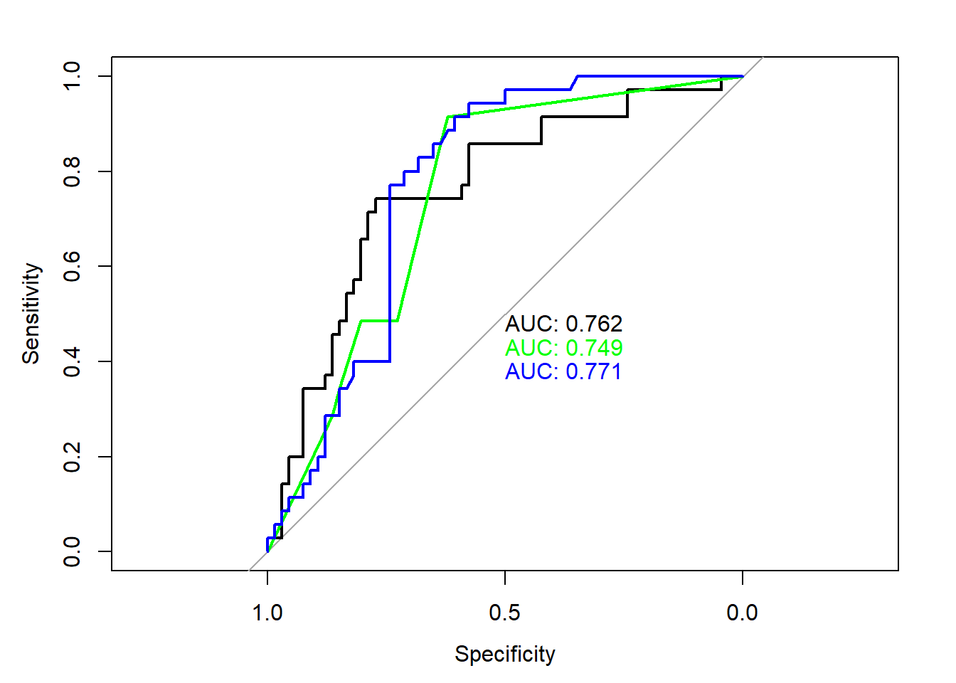

Based on AUC, perhaps logistic regression or random forest is best?

Cross Validation

Note that because we are folding our data, we’re using cejst_mod, not training and testing!

Code

# set cross validation parameters
fitControl <- trainControl(method = "repeatedcv", # fast resampling method but there are many
                           number = 10,           # number of folds
                           repeats = 10,          # number of complete sets of folds to compute
                           classProbs = TRUE,     # compute probabilities, not just Yes/No
                           summaryFunction = twoClassSummary)

# run logistic regression with 10 folds across our entire dataset
log.model <- train(CFLRP ~., data = cejst_mod[,-1],
                   # automatically uses family=binomial() for binary factor
                   method = "glm",
                   trControl = fitControl)

Warning in train.default(x, y, weights = w, ...): The metric "Accuracy" was not
in the result set. ROC will be used instead.

Code

# generate predictions for testing data
pred.log <- predict(log.model, newdata = testing, type="prob")[,2]

# run tree model with 10 folds across our entire dataset
tree.model <- train(CFLRP ~., data = cejst_mod[,-1],
                    method = "rpart",
                    trControl = fitControl)

Warning in train.default(x, y, weights = w, ...): The metric "Accuracy" was not
in the result set. ROC will be used instead.

Code

pred.tree <- predict(tree.model, newdata=testing, type="prob")[,2]

# random forest with 10 folds across our entire dataset
rf.model <- train(CFLRP ~., data = cejst_mod[,-1],
                  method = "rf",
                  trControl = fitControl)

Warning in train.default(x, y, weights = w, ...): The metric "Accuracy" was not
in the result set. ROC will be used instead.

Code

pred.rf <- predict(rf.model, newdata=testing, type="prob")[,2]

plot(roc(testing$CFLRP, pred.log), print.auc=TRUE)
plot(roc(testing$CFLRP, pred.tree), print.auc=TRUE, print.auc.y = 0.45, col="green", add=TRUE)
plot(roc(testing$CFLRP, pred.rf), print.auc=TRUE, print.auc.y = 0.4, col="blue", add=TRUE)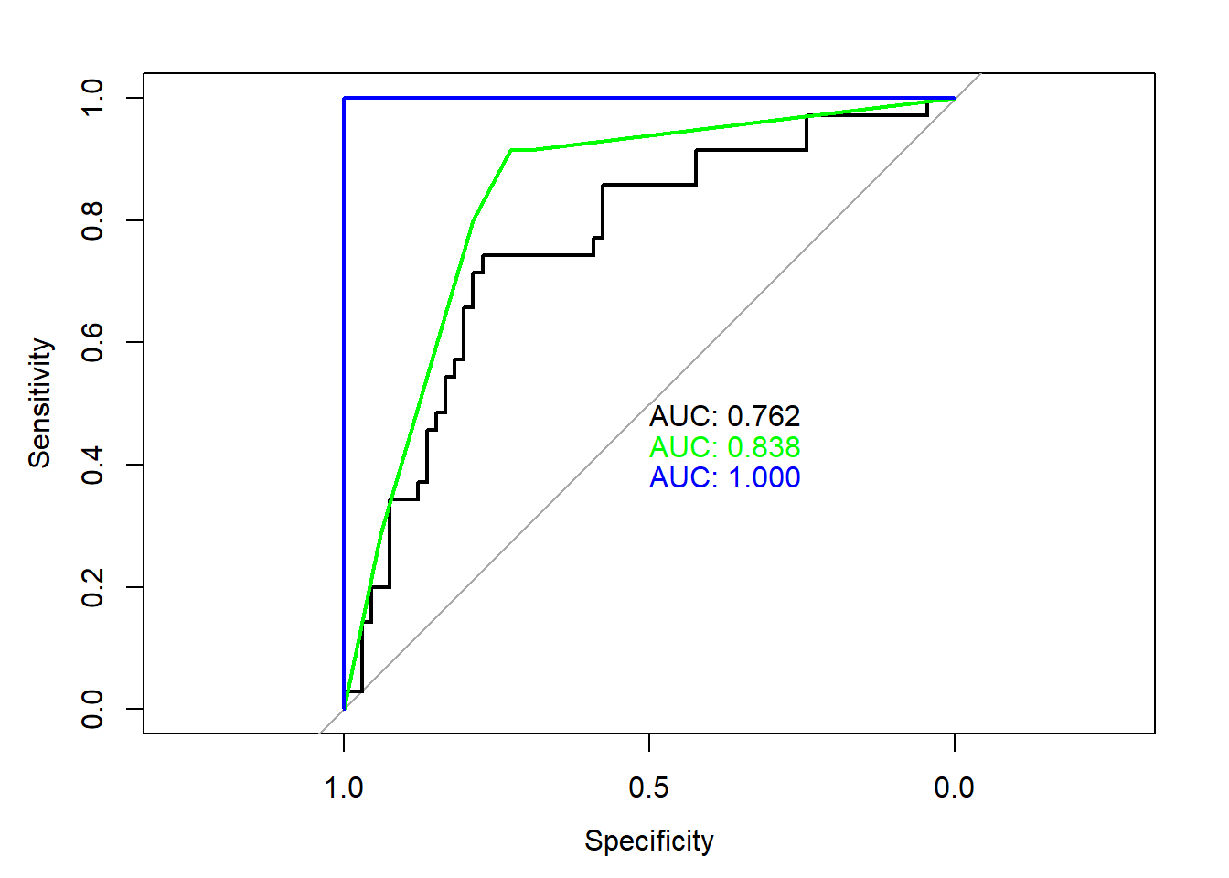

Based on cross validation (which is more robust than simple test/train splitting), random forest seems best.

Plotting the “best” model

Get best models (highest AUC values came from cross-validation models):

Code

best.rf <- rf.model$finalModel
best.log <- log.model$finalModel
best.tree <- tree.model$finalModel

We can generate predictions for the vector data or convert to raster. I’ll show both ways here for all models.

Predictions and Plotting for Vector Data

Code

log.preds <- predict(object=best.log, newdata=cejst_mod, type="response")
tree.preds <- predict(object=best.tree, newdata=cejst_mod, type="class")
rf.preds <- predict(object=best.rf, newdata=cejst_mod, type="prob")[,"Yes"]

# get geometries back for plotting predictions
cejst_pred <- left_join(cejst_mod, cejst_sub[,c("GEOID10")]) %>%
  st_as_sf(., crs = st_crs(cejst_sub)) %>%
  # join predictions
  mutate(logistic = log.preds,
         # convert to numbers for plotting
         tree = ifelse(tree.preds=="Yes", 1, 0),
         rf = rf.preds)

Joining with `by = join_by(GEOID10)`

Code

# convert data to long format for mapping
forest.cejst.long <- cejst_pred %>% 
  pivot_longer(., cols =logistic:rf, names_to="model", values_to = "pred")

tm_shape(forest.cejst.long) +
  tm_fill(col="pred") +
  tm_facets(by = c("model"), free.scales.fill = TRUE) +
  tm_shape(cflrp.bdry_sub) +
  tm_borders(col="black", lwd=1.5)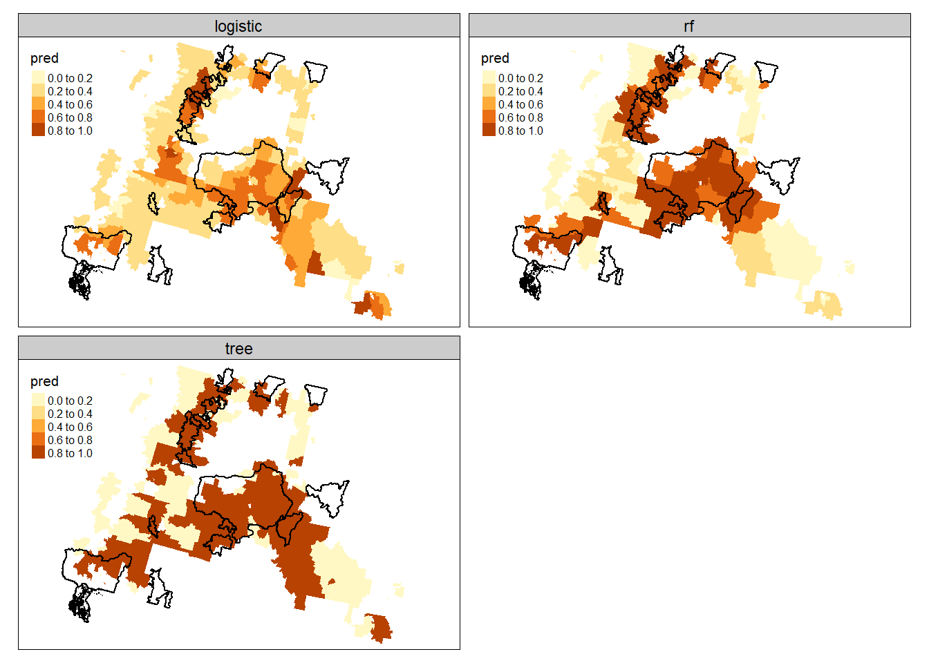

Predictions and Plotting for Raster Data

modified 11/12/24

Code

# using wildfire raster as a template to rasterize all other predictors
pred.stack <- c((rasterize(cejst_sub, wildfire_haz, field = "LMI_PFS", "mean") - mean(cejst_sub$LMI_PFS, na.rm=TRUE))/sd(cejst_sub$LMI_PFS, na.rm=TRUE),
                (rasterize(cejst_sub, wildfire_haz, field = "LHE", "mean") - mean(cejst_sub$LHE, na.rm=TRUE))/sd(cejst_sub$LHE, na.rm=TRUE),
                (rasterize(cejst_sub, wildfire_haz, field = "HBF_PFS", "mean") - mean(cejst_sub$HBF_PFS, na.rm=TRUE))/sd(cejst_sub$HBF_PFS, na.rm=TRUE),
                (wildfire_haz - mean(cejst_sub$WHP_ID, na.rm=TRUE))/sd(cejst_sub$WHP_ID, na.rm=TRUE))
plot(pred.stack)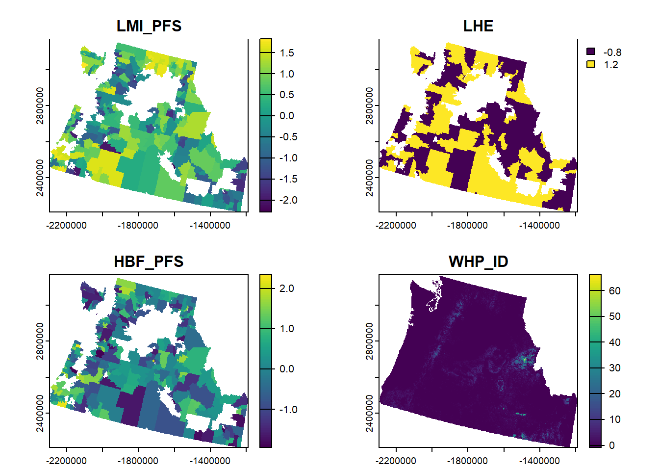

Code

log.preds_r <- terra::predict(pred.stack, best.log, type="response")


|---------|---------|---------|---------|
=========================================

Code

tree.preds_r <- terra::predict(pred.stack, best.tree, type="class")


|---------|---------|---------|---------|
=========================================

Code

# random forest doesn't like NAs, so we will replace them with 0 and then mask them out later
pred.stack_rf <- ifel(is.na(pred.stack), 0, pred.stack)


|---------|---------|---------|---------|
=========================================
                                          

|---------|---------|---------|---------|
=========================================
                                          

|---------|---------|---------|---------|
=========================================
                                          

|---------|---------|---------|---------|
=========================================
                                          

|---------|---------|---------|---------|
=========================================

Code

rf.preds_r <- terra::predict(pred.stack_rf, best.rf, type="prob")[["Yes"]]


|---------|---------|---------|---------|
=========================================

Code

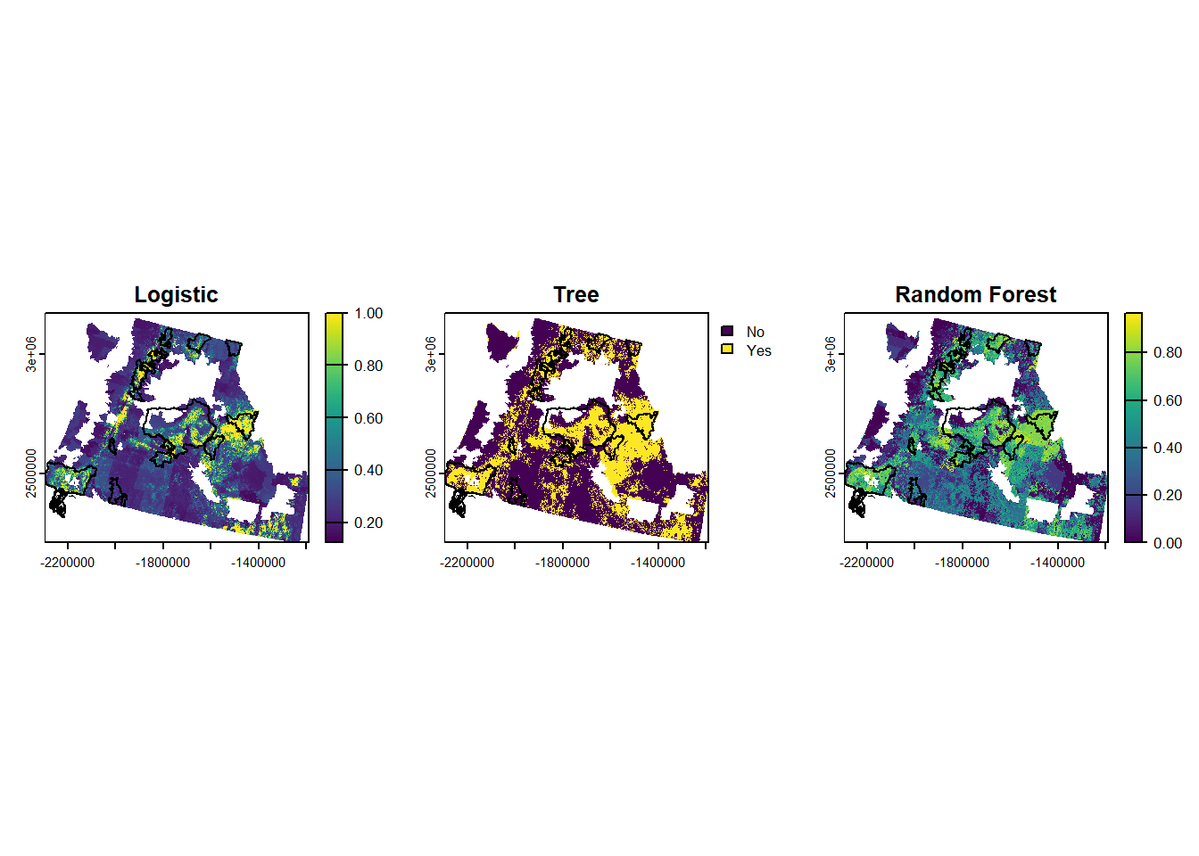
results <- c(log.preds_r, tree.preds_r, rf.preds_r)
names(results) <- c("Logistic", "Tree", "Random Forest")
results <- mask(results, cejst_sub)


|---------|---------|---------|---------|
=========================================

Code

par(mfrow=c(1,3))
plot(results[[1]], main="Logistic")
plot(st_geometry(cflrp.bdry_sub), add=TRUE)
plot(results[[2]], main="Tree")
plot(st_geometry(cflrp.bdry_sub), add=TRUE)
plot(results[[3]], main="Random Forest")
plot(st_geometry(cflrp.bdry_sub), add=TRUE)