Code
library(sf)
library(spdep)
library(tidyverse)
library(tmap)
Load libraries:
library(sf)
library(spdep)
library(tidyverse)
library(tmap)Load data:
cdc <- read_sf("/opt/data/data/vectorexample/cdc_nw.shp") %>%
  select(stateabbr, countyname, countyfips, casthma_cr)

plot(cdc["casthma_cr"])nb.qn <- poly2nb(cdc, queen = TRUE)
nb.rk <- poly2nb(cdc, queen = FALSE)visualize
par(mfrow=c(1,2))
plot(st_geometry(cdc), border = 'lightgrey')
plot(nb.qn, st_coordinates(st_centroid(cdc)), add=TRUE, col='red', main="Queen's case")
plot(st_geometry(cdc), border = 'lightgrey')
plot(nb.rk, st_coordinates(st_centroid(cdc)), add=TRUE, col='blue', main="Rook's case")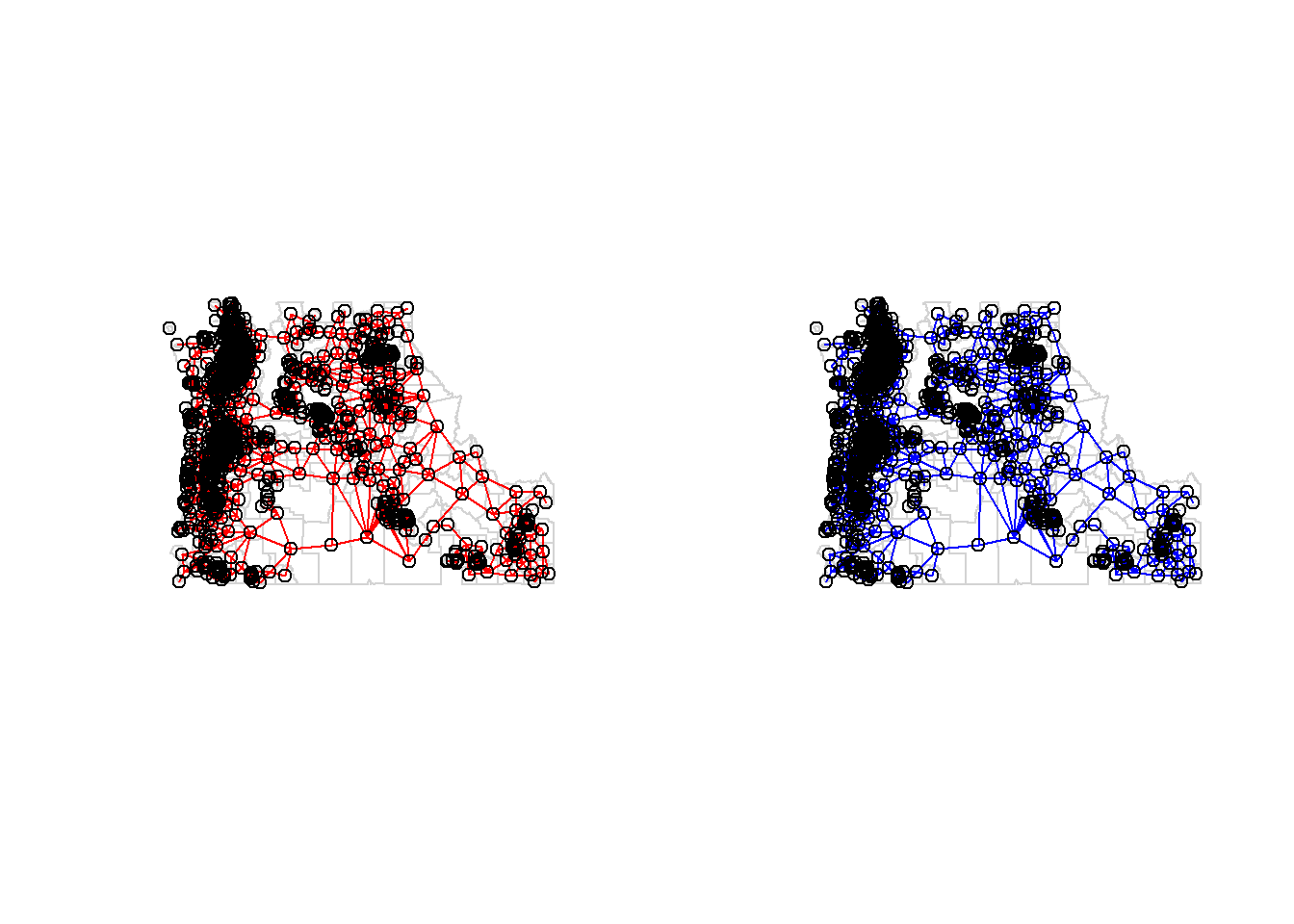
par(mfrow=c(1,1))lw.qn <- nb2listw(nb.qn, style="W", zero.policy = TRUE)
lw.qn$weights[1:5][[1]]
[1] 0.5 0.5
[[2]]
[1] 0.25 0.25 0.25 0.25
[[3]]
[1] 0.2 0.2 0.2 0.2 0.2
[[4]]
[1] 0.3333333 0.3333333 0.3333333
[[5]]
[1] 1asthma.lag <- lag.listw(lw.qn, cdc$casthma_cr)
head(asthma.lag)[1] 10.30000 9.57500 9.88000 10.26667 9.50000 9.90000M <- lm(asthma.lag ~ cdc$casthma_cr)
M
Call:
lm(formula = asthma.lag ~ cdc$casthma_cr)

Coefficients:
   (Intercept)  cdc$casthma_cr
3.7209 0.6357 plot(x = cdc$casthma_cr, y = asthma.lag)
abline(M$coefficients[1], M$coefficients[2], col="red")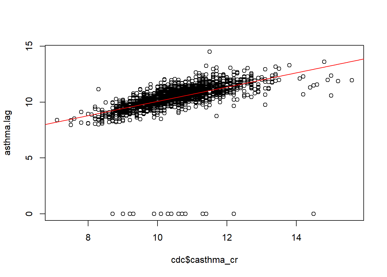
n <- 400L   # Define the number of simulations
I.r <- vector(length=n)  # Create an empty vector

for (i in 1:n){
  # Randomly shuffle asthma values
  x <- sample(cdc$casthma_cr, replace=FALSE)
  # Compute new set of lagged values
  x.lag <- lag.listw(lw.qn, x)
  # Compute the regression slope and store its value
  M.r    <- lm(x.lag ~ x)
  I.r[i] <- coef(M.r)[2]
}moran.test uses a few key assumptions, including that the data is normally distributed
moran.test(cdc$casthma_cr, lw.qn)
    Moran I test under randomisation

data:  cdc$casthma_cr
weights: lw.qn
n reduced by no-neighbour observations

Moran I statistic standard deviate = 40.826, p-value < 2.2e-16
alternative hypothesis: greater
sample estimates:
Moran I statistic       Expectation          Variance
0.6381428057 -0.0005037783 0.0002447034 cdc.pt <- st_point_on_surface(cdc)Warning: st_point_on_surface assumes attributes are constant over geometriesWarning in st_point_on_surface.sfc(st_geometry(x)): st_point_on_surface may not
give correct results for longitude/latitude data# another option is st_centroid
# get nearest neighbor for each point
geog.nearnb <- knn2nb(knearneigh(cdc.pt, k=1))
# get list of nearest neighbors so that every tract has at least one neighbor
nb.nearest <- dnearneigh(cdc.pt,
d1 = 0,
d2 = max(unlist(nbdists(geog.nearnb, cdc.pt))))lw.nearest <- nb2listw(nb.nearest, style="W")
asthma.lag <- lag.listw(lw.nearest, cdc$casthma_cr)M2 <- lm(asthma.lag ~ cdc$casthma_cr)
M2
Call:
lm(formula = asthma.lag ~ cdc$casthma_cr)

Coefficients:
   (Intercept)  cdc$casthma_cr
        8.8547          0.1578
visualize:
plot(x = cdc$casthma_cr, y = asthma.lag)
abline(M2$coefficients[1], M2$coefficients[2], col="red")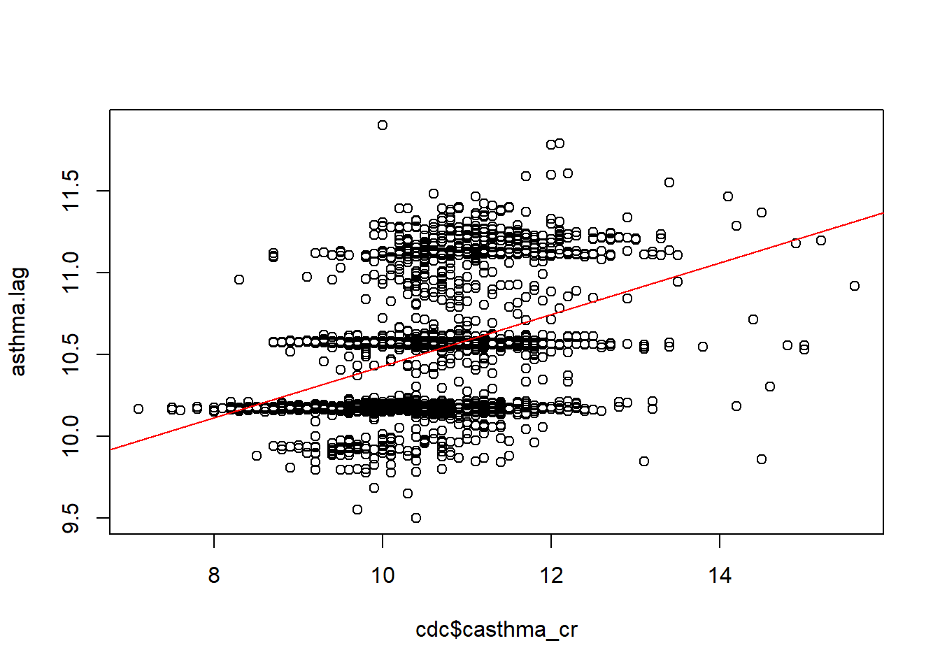
n <- 400L   # Define the number of simulations
I.r <- vector(length=n)  # Create an empty vector

for (i in 1:n){
  # Randomly shuffle asthma values
  x <- sample(cdc$casthma_cr, replace=FALSE)
  # Compute new set of lagged values - use new neighbors!
  x.lag <- lag.listw(lw.nearest, x)
  # Compute the regression slope and store its value
  M.r    <- lm(x.lag ~ x)
  I.r[i] <- coef(M.r)[2]
}i <- 1
I.r <- vector(length=n) # Create an empty vector
# Randomly shuffle asthma values
x <- sample(cdc$casthma_cr, replace=FALSE)
random_data <- cbind(cdc, x)
plot(random_data["x"])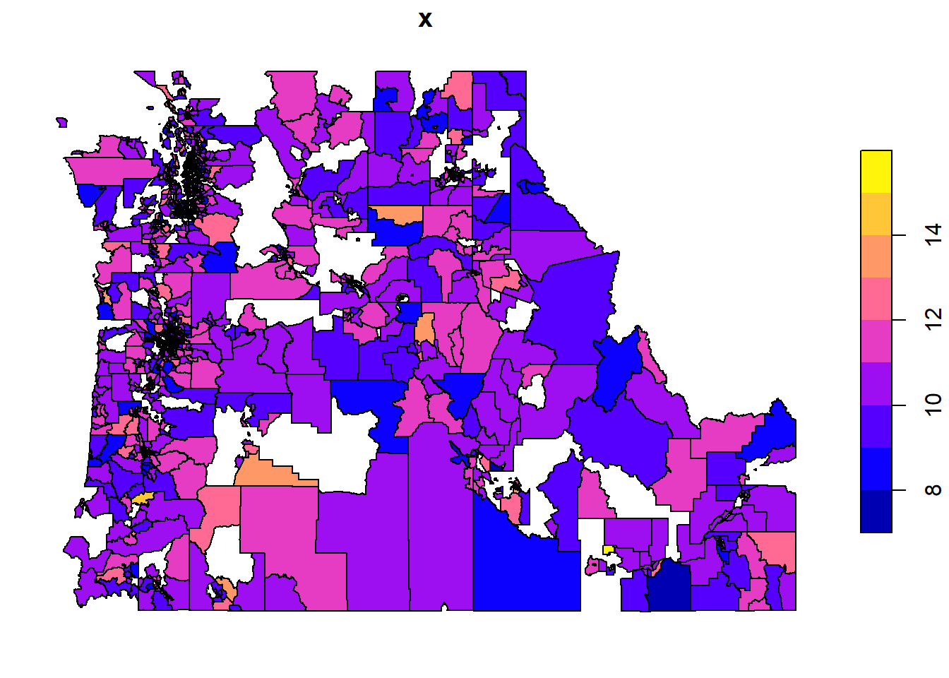
# Compute new set of lagged values
x.lag <- lag.listw(lw.nearest, x)

head(x.lag)
[1] 10.61818 10.50821 10.51805 10.48258 10.45769 10.51111# Compute the regression slope and store its value
M.r <- lm(x.lag ~ x)
I.r[i] <- coef(M.r)[2]
head(I.r)[1] -0.002479055 0.000000000 0.000000000 0.000000000 0.000000000
[6] 0.000000000cejst <- st_read("/opt/data/data/assignment01/cejst_nw.shp")
cejst.id <- cejst %>%
filter(SF == "Idaho") %>%
select(CF, SF, EPLR_PFS)After this, we tried our hand at tackling the homework questions with the cejst data individually.
Use the nearest-neighbor approach that we used in class to estimate the lagged values for the cejst dataset and estimate the slope of the line describing Moran’s I statistic.
Now use the permutation approach to compare your measured value to one generated from multiple simulations. Generate the plot of the data. Do you see more evidence of spatial autocorrelation?